


Average
In mathematics, an average of a collection or group is a value that is most central, common, or typical in some sense, and represents its overall position. In mathematics, it most commonly refers to the arithmetic mean, but may also refer to other measures such as other types of mean, the median, or the mode.
A mean is a quantity representing the "center" of a collection of numbers and is intermediate to the extreme values of the set of numbers.[1] There are several kinds of means (or "measures of central tendency") in mathematics, especially in statistics. Each attempts to summarize or typify a given group of data, illustrating the magnitude and sign of the data set. Which of these measures is most illuminating depends on what is being measured, and on context and purpose.[2]
Definitions
[edit]

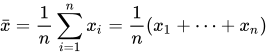
The most commonly used definition of the average is the arithmetic mean,[4] also known as "arithmetic average" i.e. the sum divided by the count, so the "average" of the list of numbers [2, 3, 4, 7, 9] is generally considered to be (2+3+4+7+9)/5 = 25/5 = 5. The arithmetic mean of a set of numbers x1, x2, ..., xn is typically denoted using an overhead bar, .[note 1] If the numbers are from observing a sample of a larger group, the arithmetic mean is termed the sample mean () to distinguish it from the group mean (or expected value) of the underlying distribution, denoted or .[note 2][5]


However, other meanings are sometimes used depending on the context, which can lead to confusion; for instance, in teaching, "average" sometimes refers to "the three Ms": mean, median, and mode.[6][7][8][9][10][11][12]
The median, defined as the value in the center after sorting the group, is usually used as the average in situations where the data is skewed or has outliers, in order to focus on the main part of the group rather than the long tail. For example, the average personal income is usually given as the median income, so that it represents the majority of the population rather than being overly influenced by the much higher incomes of the few rich people.[13]
The harmonic mean, defined as the reciprocal of the mean of the reciprocals, is used in a variety of situations involving rates or ratios, such as computing the average speed from multiple measurements taken over the same distance.[14] Indeed, unlike an arithmetic mean or median of speeds, a harmonic mean of speeds will give the value of the constant speed that would cause one to travel the same distance in the same amount of time.
The mode represents the most common value found in the group. It can be used when the data is categorical rather than numeric,[15] when the frequency of each value is relevant (such as where a histogram, bar chart, or probability density function is being referenced),[16] or to find a value that represents the majority of the group.[17]
Other statistics that can be used as an average include the mid-range, the quadratic mean or the geometric mean, but they are rarely referred to as "the average".
Central tendency
[edit]In statistics, a central tendency (or measure of central tendency) is a central or typical value for a probability distribution.[18] Informally, measures of central tendency are often called 'averages'. The term central tendency dates from the late 1920s.[19]
The most common measures of central tendency are the arithmetic mean, the median, and the mode. A middle tendency can be calculated for either a finite set of values or for a theoretical distribution, such as the normal distribution. Occasionally authors use central tendency to denote "the tendency of quantitative data to cluster around some central value."[19][20]
The central tendency of a distribution is typically contrasted with its dispersion or variability; dispersion and central tendency are the often characterized properties of distributions. Analysis may judge whether data has a strong or a weak central tendency based on its dispersion.
General properties
[edit]All averages of a collection are somewhere within its bounding box (and so for real numbers, between its maximum and minimum). Therefore, if a collection consists entirely of the same value, any average of it is that value.[21]
Most averages[a] are monotonic, i.e. moving a member of it in one direction causes the average to move in the same direction, or equivalently, if two collections of numbers A and B have the same number of elements, and they can be arranged such that each entry in A ≥ the corresponding entry in B, then the average of A ≥ the average of B.
All commonly-used averages are linearly homogeneous, i.e. multiplying every value by the same scale factor multiplies the average by that same scale factor.
Most averages[b] remain identical when the list of items is permuted, i.e. the ordering does not matter.
Statistical location
[edit]

In descriptive statistics, the mean may be confused with the median, mode or mid-range, as any of these may colloquially be called an "average" (more formally, a measure of central tendency). The mean of a set of observations is the arithmetic average of the values; however, for skewed distributions, the mean is not necessarily the same as the middle value (median), or the most likely value (mode). For example, mean income is typically skewed upwards by a small number of people with very large incomes, so that the majority have an income lower than the mean. By contrast, the median income is the level at which half the population is below and half is above. The mode income is the most likely income and favors the larger number of people with lower incomes. While the median and mode are often more intuitive measures for such skewed data, many skewed distributions are in fact best described by their mean, including the exponential and Poisson distributions.
Mean of a probability distribution
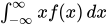
[edit]The mean of a probability distribution is the long-run arithmetic average value of a random variable having that distribution. If the random variable is denoted by , then the mean is also known as the expected value of (denoted ). For a discrete probability distribution, the mean is given by , where the sum is taken over all possible values of the random variable and is the probability mass function. For a continuous distribution, the mean is , where is the probability density function.[23] In all cases, including those in which the distribution is neither discrete nor continuous, the mean is the Lebesgue integral of the random variable with respect to its probability measure. The mean need not exist or be finite; for some probability distributions the mean is infinite (+∞ or −∞), while for others the mean is undefined.



Relationships between the mean, median and mode
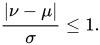
[edit]For unimodal distributions the following bounds are known and are sharp:[24]
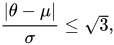
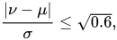
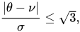
where μ is the mean, ν is the median, θ is the mode, and σ is the standard deviation.
For every distribution,[25][26]
Possible averages
[edit]| Name | Equation or description | As solution to optimization problem |
|---|---|---|
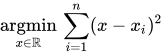
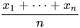
| Arithmetic mean (AM) | For example, the arithmetic mean of five values: 4, 36, 45, 50, 75 is: | |
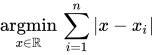
| Median | A middle value that separates the higher half from the lower half of the data set; may not be unique if the data set contains an even number of points | |
| Geometric median | A rotation invariant extension of the median for points in | |
| Tukey median | Another rotation invariant extension of the median for points in —a point that maximizes the Tukey depth | |
| Mode | The most frequent value in the data set | |
| Geometric mean (GM) | an average that is useful for sets of positive numbers, interpreted according to their product and not their sum[1] For example, the geometric mean of five values: 4, 36, 45, 50, 75 is: | |
| Harmonic mean (HM) | For example, the harmonic mean of the five values: 4, 36, 45, 50, 75 is | |
| Contraharmonic mean | ||
| Lehmer mean | ||
| Quadratic mean (or RMS) | ||
| Cubic mean | ||
| Generalized mean | ||
| Quasi-arithmetic mean | is monotonic | |
| Weighted mean | ||
| Truncated mean | The arithmetic mean of data values after a certain number or proportion of the highest and lowest data values have been discarded | |
| Interquartile mean | A special case of the truncated mean, using the interquartile range. A special case of the inter-quantile truncated mean, which operates on quantiles (often deciles or percentiles) that are equidistant but on opposite sides of the median. | |
| Midrange | ||
| Winsorized mean | Similar to the truncated mean, but, rather than deleting the extreme values, they are set equal to the largest and smallest values that remain | |
| Medoid | A representative object of a set of objects with minimal sum of dissimilarities to all the objects in the set, according to some dissimilarity function . |


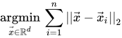

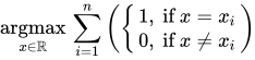
![{\displaystyle {\sqrt[{n}]{\prod _{i=1}^{n}x_{i}}}={\sqrt[{n}]{x_{1}\cdot x_{2}\dotsb x_{n}}}}](https://wikimedia.org/api/rest_v1/media/math/render/svg/a3740b9924a63fcde06a3fd26d9691c082910d78)
![{\displaystyle (4\times 36\times 45\times 50\times 75)^{\frac {1}{5}}={\sqrt[{5}]{24\;300\;000}}=30.}](https://wikimedia.org/api/rest_v1/media/math/render/svg/3b516046ef2a7b8b23301b7ab228cec73f38e062)



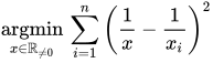



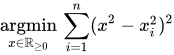
![{\displaystyle {\sqrt[{3}]{{\frac {1}{n}}\sum _{i=1}^{n}x_{i}^{3}}}={\sqrt[{3}]{{\frac {1}{n}}\left(x_{1}^{3}+x_{2}^{3}+\cdots +x_{n}^{3}\right)}}}](https://wikimedia.org/api/rest_v1/media/math/render/svg/87ea526bc6b48f6abb52bc522d57c9fedacbaf90)

![{\displaystyle {\sqrt[{p}]{{\frac {1}{n}}\cdot \sum _{i=1}^{n}x_{i}^{p}}}}](https://wikimedia.org/api/rest_v1/media/math/render/svg/b914d893b094e9e15a5681ef60069e9e5fac54ab)








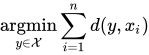
Even though perhaps not an average, the th quantile (another summary statistic that generalizes the median) can similarly be expressed as a solution to the optimization problem

- ,

which aims to minimize the total tilted absolute value loss (or quantile loss or pinball loss).
Other more sophisticated averages are: trimmore sophistiean, trimedian, and normalized mean, with their generalizations.[27]
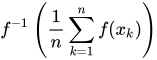
In a more general fashion, one can create their own average metric using the generalized f-mean:
![{\displaystyle y=f^{-1}\left({\frac {1}{n}}\left[f(x_{1})+f(x_{2})+\cdots +f(x_{n})\right]\right)}](https://wikimedia.org/api/rest_v1/media/math/render/svg/5fea48be50f3fe5836ae433848e3e4ca0c9827a5)
where f is any invertible function. The harmonic mean is an example of this using f(x) = 1/x, and the geometric mean is another, using f(x) = log x.
However, this method for generating means is not general enough to capture all averages. A more general method[28][failed verification] for defining an average takes any function g(x1, x2, ..., xn) of a list of arguments that is continuous, strictly increasing in each argument, and symmetric (invariant under permutation of the arguments). The average y is then the value that, when replacing each member of the list, results in the same function value: g(y, y, ..., y) = g(x1, x2, ..., xn). This most general definition still captures the important property of all averages that the average of a list of identical elements is that element itself. The function g(x1, x2, ..., xn) = x1+x2+ ··· + xn provides the arithmetic mean. The function g(x1, x2, ..., xn) = x1x2···xn (where the list elements are positive numbers) provides the geometric mean. The function g(x1, x2, ..., xn) = (x1−1+x2−1+ ··· + xn−1)−1) (where the list elements are positive numbers) provides the harmonic mean.[28]
Pythagorean means
[edit]In mathematics, the three classical Pythagorean means are the arithmetic mean (AM), the geometric mean (GM), and the harmonic mean (HM). These means were studied with proportions by Pythagoreans and later generations of Greek mathematicians[29] because of their importance in geometry and music.
Relationship between AM, GM, and HM
[edit]
PR is the diameter of a circle centered on O; its radius AO is the arithmetic mean of a and b. Triangle PGR is a right triangle from Thales's theorem, enabling use of the geometric mean theorem to show that its altitude GQ is the geometric mean. For any ratio a:b, AO ≥ GQ.
AM, GM, and HM of nonnegative real numbers satisfy these inequalities:[30]

Equality holds if all the elements of the given sample are equal.
Power mean
[edit]The generalized mean, also known as the power mean or Hölder mean, abstracts several other means. It is defined for positive numbers by[1]


This, as a function of , is well defined on , but can be extended continuously to .[31] By choosing different values for , other well known means are retrieved.



| Name | Exponent | Value |
|---|---|---|
| Minimum | ||
| Harmonic mean | ||
| Geometric mean | ||
| Arithmetic mean | ||
| Root mean square | ||
| Cubic mean | ||
| Maximum |




![{\displaystyle {\sqrt[{n}]{x_{1}\dots x_{n}}}}](https://wikimedia.org/api/rest_v1/media/math/render/svg/1af36d22e6641f7ad5ac4cb1973aed19f22c360f)



![{\displaystyle {\sqrt[{3}]{\frac {x_{1}^{3}+\dots +x_{n}^{3}}{n}}}}](https://wikimedia.org/api/rest_v1/media/math/render/svg/e82e4236bdf98c1e7d86ce7b481d2c49d34a4676)


Quasi-arithmetic mean
[edit]A similar approach to the power mean is the -mean, also known as the quasi-arithmetic mean. For an injective function on an interval and real numbers we define their -mean as




By choosing different functions , other well known means are retrieved.
| Mean | Function[note 3] | |
|---|---|---|
| Arithmetic mean | ||
| Geometric mean | [note 4] | |
| Harmonic mean | ||
| Power mean | [note 5] |


![{\displaystyle ]0,+\infty [}](https://wikimedia.org/api/rest_v1/media/math/render/svg/e91ea5ab8b69e30f90c2bdf5db4b620815bde815)


Weighted arithmetic mean
[edit]The weighted arithmetic mean (or weighted average) is used if one wants to combine average values from different sized samples of the same population, and is define by[1]

where and are the mean and size of sample respectively. In other applications, they represent a measure for the reliability of the influence upon the mean by the respective values.


Truncated mean
[edit]Sometimes, a set of numbers might contain outliers. Often, outliers are erroneous data caused by artifacts. In this case, one can use a truncated mean. It involves discarding given parts of the data at the top or the bottom end, typically an equal amount at each end and then taking the arithmetic mean of the remaining data. A specific example of a truncated mean is the interquartile mean.
Mean of a function
[edit]In some circumstances, mathematicians may calculate a mean of an infinite (or even an uncountable) set of values. This can happen when calculating the mean value of a function . Intuitively, a mean of a function can be thought of as calculating the area under a section of a curve, and then dividing by the length of that section. This can be done crudely by counting squares on graph paper, or more precisely by integration. The integration formula is written as:


In this case, care must be taken to make sure that the integral converges. But the mean may be finite even if the function itself tends to infinity at some points.
Mean of angles and cyclical quantities
[edit]Angles, times of day, and other cyclical quantities require modular arithmetic to add and otherwise combine numbers. These quantities can be averaged using the circular mean. In all these situations, it is possible that no mean exists, for example if all points being averaged are equidistant. Consider a color wheel—there is no mean to the set of all colors. Additionally, there may not be a unique mean for a set of values: for example, when averaging points on a clock, the mean of the locations of 11:00 and 13:00 is 12:00, but this location is equivalent to that of 00:00.
Fréchet mean
[edit]The Fréchet mean gives a manner for determining the "center" of a mass distribution on a surface or, more generally, Riemannian manifold. Unlike many other means, the Fréchet mean is defined on a space whose elements cannot necessarily be added together or multiplied by scalars.
Center of a triangle
[edit]In geometry, there are thousands of different definitions for the center of a triangle that can all be interpreted as the mean of a triangular set of points in the plane.[32]
Swanson's rule
[edit]This is an approximation to the mean for a moderately skewed distribution.[33] It is used in hydrocarbon exploration and is defined as:

where , and are the 10th, 50th and 90th percentiles of the distribution, respectively.


Moving average
[edit]Given a time series, such as daily stock market prices or yearly temperatures, people often want to create a smoother series.[34] This helps to show underlying trends or perhaps periodic behavior. An easy way to do this is the moving average: one chooses a number n and creates a new series by taking the arithmetic mean of the first n values, then moving forward one place by dropping the oldest value and introducing a new value at the other end of the list, and so on. This is the simplest form of moving average. More complicated forms involve using a weighted average. The weighting can be used to enhance or suppress various periodic behaviors and there is extensive analysis of what weightings to use in the literature on filtering. In digital signal processing the term "moving average" is used even when the sum of the weights is not 1.0 (so the output series is a scaled version of the averages).[35] The reason for this is that the analyst is usually interested only in the trend or the periodic behavior.
Solutions to variational problems
[edit]Several measures of central tendency can be characterized as solving a variational problem, in the sense of the calculus of variations, namely minimizing variation from the center. That is, given a measure of statistical dispersion, one asks for a measure of central tendency that minimizes variation: such that variation from the center is minimal among all choices of center. In a quip, "dispersion precedes location". These measures are initially defined in one dimension, but can be generalized to multiple dimensions. This center may or may not be unique. In the sense of Lp spaces, the correspondence is:
| Lp | dispersion | central tendency |
|---|---|---|
| L0 | variation ratio | mode[c] |
| L1 | average absolute deviation | median (geometric median)[d] |
| L2 | standard deviation | mean (centroid)[e] |
| L∞ | maximum deviation | midrange[f] |
The associated functions are called p-norms: respectively 0-"norm", 1-norm, 2-norm, and ∞-norm. The function corresponding to the L0 space is not a norm, and is thus often referred to in quotes: 0-"norm".
In equations, for a given (finite) data set X, thought of as a vector x = (x1,…,xn), the dispersion about a point c is the "distance" from x to the constant vector c = (c,…,c) in the p-norm (normalized by the number of points n):

For p = 0 and p = ∞ these functions are defined by taking limits, respectively as p → 0 and p → ∞. For p = 0 the limiting values are 00 = 0 and a0 = 1 for a ≠ 0, so the difference becomes simply equality, so the 0-norm counts the number of unequal points. For p = ∞ the largest number dominates, and thus the ∞-norm is the maximum difference.
Uniqueness
[edit]The mean (L2 center) and midrange (L∞ center) are unique (when they exist), while the median (L1 center) and mode (L0 center) are not in general unique. This can be understood in terms of convexity of the associated functions (coercive functions).
The 2-norm and ∞-norm are strictly convex, and thus (by convex optimization) the minimizer is unique (if it exists), and exists for bounded distributions. Thus standard deviation about the mean is lower than standard deviation about any other point, and the maximum deviation about the midrange is lower than the maximum deviation about any other point.
The 1-norm is not strictly convex, whereas strict convexity is needed to ensure uniqueness of the minimizer. Correspondingly, the median (in this sense of minimizing) is not in general unique, and in fact any point between the two central points of a discrete distribution minimizes average absolute deviation.
The 0-"norm" is not convex (hence not a norm). Correspondingly, the mode is not unique – for example, in a uniform distribution any point is the mode.
Clustering
[edit]Instead of a single central point, one can ask for multiple points such that the variation from these points is minimized. This leads to cluster analysis, where each point in the data set is clustered with the nearest "center". Most commonly, using the 2-norm generalizes the mean to k-means clustering, while using the 1-norm generalizes the (geometric) median to k-medians clustering. Using the 0-norm simply generalizes the mode (most common value) to using the k most common values as centers.
Unlike the single-center statistics, this multi-center clustering cannot in general be computed in a closed-form expression, and instead must be computed or approximated by an iterative method; one general approach is expectation–maximization algorithms.
Information geometry
[edit]The notion of a "center" as minimizing variation can be generalized in information geometry as a distribution that minimizes divergence (a generalized distance) from a data set. The most common case is maximum likelihood estimation, where the maximum likelihood estimate (MLE) maximizes likelihood (minimizes expected surprisal), which can be interpreted geometrically by using entropy to measure variation: the MLE minimizes cross-entropy (equivalently, relative entropy, Kullback–Leibler divergence).
A simple example of this is for the center of nominal data: instead of using the mode (the only single-valued "center"), one often uses the empirical measure (the frequency distribution divided by the sample size) as a "center". For example, given binary data, say heads or tails, if a data set consists of 2 heads and 1 tails, then the mode is "heads", but the empirical measure is 2/3 heads, 1/3 tails, which minimizes the cross-entropy (total surprisal) from the data set. This perspective is also used in regression analysis, where least squares finds the solution that minimizes the distances from it, and analogously in logistic regression, a maximum likelihood estimate minimizes the surprisal (information distance).
History
[edit]Origin
[edit]The first recorded time that the arithmetic mean was extended from 2 to n cases for the use of estimation was in the sixteenth century. From the late sixteenth century onwards, it gradually became a common method to use for reducing errors of measurement in various areas.[36][37] At the time, astronomers wanted to know a real value from noisy measurement, such as the position of a planet or the diameter of the moon. Using the mean of several measured values, scientists assumed that the errors add up to a relatively small number when compared to the total of all measured values. The method of taking the mean for reducing observation errors was mainly developed in astronomy.[36][38] A possible precursor to the arithmetic mean is the mid-range (the mean of the two extreme values), used for example in Arabian astronomy of the ninth to eleventh centuries, but also in metallurgy and navigation.[37]
However, there are various older vague references to the use of the arithmetic mean (which are not as clear, but might reasonably have to do with our modern definition of the mean). In a text from the 4th century, it was written that (text in square brackets is a possible missing text that might clarify the meaning):[39]
- In the first place, we must set out in a row the sequence of numbers from the monad up to nine: 1, 2, 3, 4, 5, 6, 7, 8, 9. Then we must add up the amount of all of them together, and since the row contains nine terms, we must look for the ninth part of the total to see if it is already naturally present among the numbers in the row; and we will find that the property of being [one] ninth [of the sum] only belongs to the [arithmetic] mean itself...
Even older potential references exist. There are records that from about 700 BC, merchants and shippers agreed that damage to the cargo and ship (their "contribution" in case of damage by the sea) should be shared equally among themselves.[38] This might have been calculated using the average, although there seem to be no direct record of the calculation.
Etymology
[edit]The root is found in Arabic as عوار ʿawār, a defect, or anything defective or damaged, including partially spoiled merchandise; and عواري ʿawārī (also عوارة ʿawāra) = "of or relating to ʿawār, a state of partial damage".[g] Within the Western languages the word's history begins in medieval sea-commerce on the Mediterranean. 12th and 13th century Genoa Latin avaria meant "damage, loss and non-normal expenses arising in connection with a merchant sea voyage"; and the same meaning for avaria is in Marseille in 1210, Barcelona in 1258 and Florence in the late 13th.[h] 15th-century French avarie had the same meaning, and it begot English "averay" (1491) and English "average" (1502) with the same meaning. Today, Italian avaria, Catalan avaria and French avarie still have the primary meaning of "damage". The transformation of the meaning in English began in later medieval and early modern Western merchant-marine law contracts under which if the ship met a bad storm and some of the goods had to be thrown overboard to make the ship lighter and safer, then all merchants whose goods were on the ship were to suffer proportionately (and not whoever's goods were thrown overboard); and more generally there was to be proportionate distribution of any avaria[citation needed]. From there the word was adopted by British insurers, creditors, and merchants for talking about their losses as being spread across their whole portfolio of assets and having a mean proportion.[h][40]
Marine damage is either particular average, which is borne only by the owner of the damaged property, or general average, where the owner can claim a proportional contribution from all the parties to the marine venture. The type of calculations used in adjusting general average gave rise to the use of "average" to mean "arithmetic mean".
A second English usage, documented as early as 1674 and sometimes spelled "averish", is as the residue and second growth of field crops, which were considered suited to consumption by draught animals ("avers").[41]
There is earlier (from at least the 11th century), unrelated use of the word. It appears to be an old legal term for a tenant's day labour obligation to a sheriff, probably anglicised from "avera" found in the English Domesday Book (1085).
The Oxford English Dictionary, however, says that derivations from German hafen haven, and Arabic ʿawâr loss, damage, have been "quite disposed of" and the word has a Romance origin.[42]
Averages as a rhetorical tool
[edit]Due to the aforementioned colloquial nature of the term "average", the term can be used to obfuscate the true meaning of data and suggest varying answers to questions based on the averaging method (most frequently arithmetic mean, median, or mode) used. In his article "Framed for Lying: Statistics as In/Artistic Proof", University of Pittsburgh faculty member Daniel Libertz comments that statistical information is frequently dismissed from rhetorical arguments for this reason.[43] However, due to their persuasive power, averages and other statistical values should not be discarded completely, but instead used and interpreted with caution. Libertz invites us to engage critically not only with statistical information such as averages, but also with the language used to describe the data and its uses, saying: "If statistics rely on interpretation, rhetors should invite their audience to interpret rather than insist on an interpretation."[43] In many cases, data and specific calculations are provided to help facilitate this audience-based interpretation.
See also
[edit]
- Average absolute deviation
- Central limit theorem
- Central moment
- Descriptive statistics
- Expected value
- Kurtosis
- Law of averages
- Location parameter
- Mean value theorem
- Moment (mathematics)
- Population mean
- Sample mean
- Statistical dispersion
- Summary statistics
- Taylor's law
Other means
[edit]- Arithmetic-geometric mean
- Arithmetic-harmonic mean
- Cesàro mean
- Chisini mean
- Contraharmonic mean
- Elementary symmetric mean
- Geometric-harmonic mean
- Grand mean
- Heinz mean
- Heronian mean
- Identric mean
- Lehmer mean
- Logarithmic mean
- Moving average
- Neuman–Sándor mean
- Quasi-arithmetic mean
- Root mean square (quadratic mean)
- Rényi's entropy (a generalized f-mean)
- Spherical mean
- Stolarsky mean
- Weighted geometric mean
- Weighted harmonic mean
Notes
[edit]Arabic:
- ↑ One exception to this is the mode; for example, the mode of [1, 1, 2, 2, 2] is 2, but the mode of [1, 1, 2, 3, 4] is 1. Also, most kinds of averages are strictly monotone, but some, such as the median, truncated mean, and winsorized mean, are only weakly monotone, and may remain the same after some of the values are increased.
- ↑ Exceptions to this may include weighted averages (if the weights are assigned by position) and moving averages (if the entire resulting sequence or curve is considered). Moving averages are often done using position-weighted averages.
- ↑ Unlike the other measures, the mode does not require any geometry on the set, and thus applies equally in one dimension, multiple dimensions, or even for categorical variables.
- ↑ The median is only defined in one dimension; the geometric median is a multidimensional generalization.
- ↑ The mean can be defined identically for vectors in multiple dimensions as for scalars in one dimension; the multidimensional form is often called the centroid.
- ↑ In multiple dimensions, the midrange can be define coordinate-wise (take the midrange of each coordinate), though this is not common.
- ↑ Medieval Arabic had عور ʿawr meaning "blind in one eye" and عوار ʿawār meant "any defect, or anything defective or damaged". Some medieval Arabic dictionaries are at Baheth.info Archived 2013-10-29 at the Wayback Machine, and some translation to English of what's in the medieval Arabic dictionaries is in Lane's Arabic-English Lexicon, pages 2193 and 2195. The medieval dictionaries do not list the word-form عوارية ʿawārīa. ʿAwārīa can be naturally formed in Arabic grammar to refer to things that have ʿawār, but in practice in medieval Arabic texts ʿawārīa is a rarity or non-existent, while the forms عواري ʿawārī and عوارة ʿawāra are frequently used when referring to things that have ʿawār or damage – this can be seen in the searchable collection of medieval texts at AlWaraq.net (book links are clickable on righthand side).
- 1 2 The Arabic origin of avaria was first reported by Reinhart Dozy in the 19th century. Dozy's original summary is in his 1869 book Glossaire. Summary information about the word's early records in Italian-Latin, Italian, Catalan, and French is at avarie @ CNRTL.fr Archived 2019-01-06 at the Wayback Machine. The seaport of Genoa is the location of the earliest-known record in European languages, year 1157. A set of medieval Latin records of avaria at Genoa is in the downloadable lexicon Vocabolario Ligure, by Sergio Aprosio, year 2001, avaria in Volume 1 pages 115-116. Many more records in medieval Latin at Genoa are at StoriaPatriaGenova.it, usually in the plurals avariis and avarias. At the port of Marseille in the 1st half of the 13th century notarized commercial contracts have dozens of instances of Latin avariis (ablative plural of avaria), as published in Blancard year 1884. Some information about the English word over the centuries is at NED (year 1888). See also the definition of English "average" in English dictionaries published in the early 18th century, i.e., in the time period just before the big transformation of the meaning: Kersey-Phillips' dictionary (1706), Blount's dictionary (1707 edition), Hatton's dictionary (1712), Bailey's dictionary (1726), Martin's dictionary (1749). Some complexities surrounding the English word's history are discussed in Hensleigh Wedgwood year 1882 page 11 and Walter Skeat year 1888 page 781. Today there is consensus that: (#1) today's English "average" descends from medieval Italian avaria, Catalan avaria, and (#2) among the Latins the word avaria started in the 12th century and it started as a term of Mediterranean sea-commerce, and (#3) there is no root for avaria to be found in Latin, and (#4) a substantial number of Arabic words entered Italian, Catalan and Provençal in the 12th and 13th centuries starting as terms of Mediterranean sea-commerce, and (#5) the Arabic ʿawār | ʿawārī is phonetically a good match for avaria, as conversion of w to v was regular in Latin and Italian, and -ia is a suffix in Italian, and the Western word's earliest records are in Italian-speaking locales (writing in Latin). And most commentators agree that (#6) the Arabic ʿawār | ʿawārī = "damage | relating to damage" is semantically a good match for avaria = "damage or damage expenses". A minority of commentators have been dubious about this on the grounds that the early records of Italian-Latin avaria have, in some cases, a meaning of "an expense" in a more general sense – see TLIO (in Italian). The majority view is that the meaning of "an expense" was an expansion from "damage and damage expense", and the chronological order of the meanings in the records supports this view, and the broad meaning "an expense" was never the most commonly used meaning. On the basis of the above points, the inferential step is made that the Latinate word came or probably came from the Arabic word.
Numeric:


References
[edit]- 1 2 3 4 "Mean | mathematics". Encyclopedia Britannica. Retrieved 2020-08-21.
- ↑ Why Few Math Students Actually Understand the Meaning of Means (YouTube video). Math The World. 2024-08-27. Retrieved 2024-09-10.
- ↑ Cantrell, David W. "Pythagorean Means". MathWorld. Retrieved 2025-11-04.
- ↑ Kaplan, Jennifer; Fisher, Dianne G.; Rogness, Neal T. (July 2010). "Lexical Ambiguity in Statistics: How students use and define the words: association, average, confidence, random and spread" [part 2] (PDF). Journal of Statistics Education. 18 (2). doi:10.1080/10691898.2010.11889491. eISSN 1069-1898.
- ↑ Underhill, L.G.; Bradfield d. (1998) Introstat, Juta and Company Ltd. ISBN 0-7021-3838-X p. 181
- ↑ Stack, Sue; Watson, Jane; Hindley, Sue; Samson, Pauline; Devlin, Robyn (2010). "What's average?". Australian Mathematics Teacher (AMT). 66 (3): 7–15. ISSN 0045-0685. Academia 48155690. EBSCOhost 53382428. Informit 10.3316/informit.354027435519820.
- ↑ Quinnell, Lorna (September 2017). "Those muddling M's: Scaffolding understanding of averages in mathematics". The Australian Mathematics Teacher (AMT). 73 (3): 6–12. ISSN 0045-0685. EBSCOhost 125324609. Informit 10.3316/informit.123380293707263, 10.3316/aeipt.218997.
- ↑ Watson, Jane M.; Moritz, Jonathan B. (1999). "The Development of Concepts of Average". Focus on Learning Problems in Mathematics. 21 (4): 15–39. ISSN 0272-8893. ERIC EJ612005.
- ↑ Watson, Jane M. (May 2007). "The Role of Cognitive Conflict in Developing Students' Understanding of Average". Educational Studies in Mathematics. 65: 21–47. doi:10.1007/s10649-006-9043-3. ISSN 0013-1954.
- ↑ Kaplan, Jennifer J.; Fisher, Diane G.; Rogness, Neal T. (2009). "Lexical Ambiguity in Statistics: What do students know about the words association, average, confidence, random and spread?" [part 1]. Journal of Statistics Education. 17 (3). doi:10.1080/10691898.2009.11889535. eISSN 1069-1898.
- ↑ Triola, Mario F. (2014). Elementary Statistics (PDF) (12th Pearson New International ed.). Pearson Education Limited. p. 53. ISBN 978-1-292-03941-1.
- ↑ Watson, Jane; Chick, Helen (July 2–6, 2012). Average Revisited in Context. 35th Annual Meeting of the Mathematics Education Research Group of Australasia (MERGA), Singapore. Adelaide SA, Australia: Mathematics Education Research Group of Australasia. pp. 753–760. This research was partially funded by ARC Linkage Grant No. LP0669106.
- ↑ "Mean or median? 'Average' household income". Statistics for the Terrified. Concept Stew Ltd. 4 April 2005. Archived from the original on 2005-12-05.
- ↑ de Mestre, Neville (2019). "discovery: What do you mean by an average?". Australian Mathematics Education Journal (AMEJ). 1 (4): 24–25. ISSN 2652-0176. EBSCOhost 140411813. Informit 10.3316/informit.837688193205822.
- ↑ "Teacher Discussion - Meet the Averages" [based on an article in The Mercury, Sunday, 16 August, 1998, p.9]. Numeracy in the News. Archived from the original on 2011-03-01.
- ↑ Landtblom, Karin (July 2018). Sorto, M. A.; White, A.; Guyot, L. (eds.). IS DATA A QUANTITATIVE THING? AN ANALYSIS OF THE CONCEPT OF THE MODE IN TEXTBOOKS FOR GRADE 4-6 (PDF). Tenth International Conference on Teaching Statistics (ICOTS10), Kyoto, Japan. Looking back, looking forward. Voorburg, The Netherlands: International Statistical Institute. Archived from the original (PDF) on 2019-12-18.
- ↑ Fowler, Elizabeth M. (August 4, 1956). "The Three Averages: A Study of How and Why Statisticians Make Use of Mean, Median and Mode / 3 AVERAGES USED BY STATISTICIANS". New York Times. pp. 19, 25 [but digitally tagged as 28, 34]. ProQuest 113794286.
- ↑ Weisberg H.F (1992) Central Tendency and Variability, Sage University Paper Series on Quantitative Applications in the Social Sciences, ISBN 0-8039-4007-6 p.2
- 1 2 Upton, G.; Cook, I. (2008) Oxford Dictionary of Statistics, OUP ISBN 978-0-19-954145-4 (entry for "central tendency")
- ↑ Dodge, Y. (2003) The Oxford Dictionary of Statistical Terms, OUP for International Statistical Institute. ISBN 0-19-920613-9 (entry for "central tendency")
- ↑ Nagumo, Mitio (1930) [Eingegangen am 1. November, 1929]. "9. Über eine Klasse der Mittelwerte". Japanese Journal of Mathematics. VII: 71–79. HathiTrust record 006954247, items inu.30000091433023, uc1.31822020414991, rul.39030029662022.
- ↑ "AP Statistics Review - Density Curves and the Normal Distributions". Archived from the original on 2 April 2015. Retrieved 16 March 2015.
- ↑ Weisstein, Eric W. "Population Mean". mathworld.wolfram.com. Retrieved 2020-08-21.
- ↑ Johnson NL, Rogers CA (1951) "The moment problem for unimodal distributions". Annals of Mathematical Statistics, 22 (3) 433–439
- ↑ Hotelling H, Solomons LM (1932) The limits of a measure of skewness. Annals Math Stat 3, 141–114
- ↑ Garver (1932) Concerning the limits of a mesuare of skewness. Ann Math Stats 3(4) 141–142
- ↑ Merigo, Jose M.; Cananovas, Montserrat (2009). "The Generalized Hybrid Averaging Operator and its Application in Decision Making". Journal of Quantitative Methods for Economics and Business Administration. 9: 69–84. ISSN 1886-516X.
- 1 2 Bibby, John (1974). "Axiomatisations of the average and a further generalisation of monotonic sequences". Glasgow Mathematical Journal. 15: 63–65. doi:10.1017/s0017089500002135.
- ↑ Heath, Thomas. History of Ancient Greek Mathematics.
- ↑ Djukić, Dušan; Janković, Vladimir; Matić, Ivan; Petrović, Nikola (2011-05-05). The IMO Compendium: A Collection of Problems Suggested for The International Mathematical Olympiads: 1959-2009 Second Edition. Springer Science & Business Media. ISBN 978-1-4419-9854-5.
- ↑ P. S. Bullen: Handbook of Means and Their Inequalities. Dordrecht, Netherlands: Kluwer, 2003, pp. 176.
- ↑ Narboux, Julien; Braun, David (2016). "Towards a certified version of the encyclopedia of triangle centers" (PDF). Mathematics in Computer Science. 10 (1): 57–73. doi:10.1007/s11786-016-0254-4. MR 3483261.
under the guidance of Clark Kimberling, an electronic encyclopedia of triangle centers (ETC) has been developed, it contains more than 7000 centers and many properties of these points
- ↑ Hurst A, Brown GC, Swanson RI (2000) Swanson's 30-40-30 Rule. American Association of Petroleum Geologists Bulletin 84(12) 1883-1891
- ↑ Box, George E.P.; Jenkins, Gwilym M. (1976). Time Series Analysis: Forecasting and Control (revised ed.). Holden-Day. ISBN 0-8162-1104-3.
- ↑ Haykin, Simon (1986). Adaptive Filter Theory. Prentice-Hall. ISBN 0-13-004052-5.
- 1 2 Plackett, R. L. (1958). "Studies in the History of Probability and Statistics: VII. The Principle of the Arithmetic Mean". Biometrika. 45 (1/2): 130–135. doi:10.2307/2333051. JSTOR 2333051.
- 1 2 Eisenhart, Churchill. "The development of the concept of the best mean of a set of measurements from antiquity to the present day." Unpublished presidential address, American Statistical Association, 131st Annual Meeting, Fort Collins, Colorado. 1971.
- 1 2 "Bakker, Arthur. "The early history of average values and implications for education." Journal of Statistics Education 11.1 (2003): 17-26". Archived from the original on 2015-12-04. Retrieved 2015-10-22.
- ↑ "Waterfield, Robin. "The theology of arithmetic." On the Mystical, mathematical and Cosmological Symbolism of the First Ten Number (1988). page 70" (PDF). Archived from the original (PDF) on 2016-03-04. Retrieved 2018-11-27.
- ↑ "average". Dictionary.com Unabridged (Online). n.d. Retrieved 2023-05-25.
- ↑ Ray, John (1674). A Collection of English Words not Generally Used. London: H. Bruges. Retrieved 18 May 2015.
- ↑ "average, n.2". Oxford English Dictionary (online ed.). Oxford University Press. September 2019. Retrieved September 5, 2019. (Subscription or participating institution membership required.)
- 1 2 Libertz, Daniel (2018-12-31). "Framed for Lying: Statistics as In/Artistic Proof". Res Rhetorica. 5 (4). doi:10.29107/rr2018.4.1. ISSN 2392-3113.
Further reading
[edit]- Bakker, Arthur (March 2003). "The Early History of Average Values and Implications for Education". Journal of Statistics Education. 11 (1). doi:10.1080/10691898.2003.11910694.
- Edgeworth, F. Y. (1889) [Read May 25, 1885.]. "VII. Observations and Statistics. An Essay on the Theory of Errors of Observation and the First Principles of Statistics". Transactions of the Cambridge Philosophical Society. XIV (II): 138–169. Google Books TdIsAAAAYAAJ. HathiTrust record 000526741, item mdp.39015008919659; record 100324784, item hvd.32044092879402.
- Edgeworth, F. Y. (May 25, 1885). "(4) Observations and statistics : Abstract". Proceedings of the Cambridge Philosophical Society. V (IV): 310–312. Google Books KdIsAAAAYAAJ, zpw1AAAAIAAJ. HathiTrust record 100528415, item hvd.hwhqbe. Internet Archive proceedingscambr05camb, proceedingsofcam5188386camb, proceedingscamb09socigoog.
- "Corrigendum on Mr F. Y. Edgeworth's paper". Proceedings of the Cambridge Philosophical Society. VI (II): 101–102. May 30, 1887. Google Books E501AAAAIAAJ. Internet Archive proceedingscamb12socigoog.
- Kennedy, Christopher; Stanley, Jason (July 2009). "On 'Average'". Mind. 118 (471): 583–646. doi:10.1093/mind/fzp094. eISSN 1460-2113. ISSN 0026-4423.
External links
[edit]


