// Workers AI · dad joke modeWhat did quantized state say? It's in a bit of a state.

The quantized state systems (QSS) methods are a family of numerical integration solvers based on the idea of state quantization, dual to the traditional idea of time discretization. Unlike traditional numerical solution methods, which approach the problem by discretizing time and solving for the next (real-valued) state at each successive time step, QSS methods keep time as a continuous entity and instead quantize the system's state, instead solving for the time at which the state deviates from its quantized value by a quantum.

They can also have many advantages compared to classical algorithms. They inherently allow for modeling discontinuities in the system due to their discrete-event nature and asynchronous nature. They also allow for explicit root-finding and detection of zero-crossing using explicit algorithms, avoiding the need for iteration---a fact which is especially important in the case of stiff systems, where traditional time-stepping methods require a heavy computational penalty due to the requirement to implicitly solve for the next system state. Finally, QSS methods satisfy remarkable global stability and error bounds, described below, which are not satisfied by classical solution techniques.

Theoretical properties

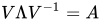
In 2001, Ernesto Kofman proved a remarkable property of the quantized-state system simulation method: namely, that when the technique is used to solve a stable linear time-invariant (LTI) system, the global error is bounded by a constant that is proportional to the quantum, but (crucially) independent of the duration of the simulation. More specifically, for a stable multidimensional LTI system with the state-transition matrix $A$ and input matrix $B$, it was shown in [CK06] that the absolute error vector ${\vec {e}}(t)$ is bounded above by

$\left|{\vec {e}}(t)\right|\leq \left|V\right|\ \left|\Re \left(\Lambda \right)^{-1}\Lambda \right|\ \left|V^{-1}\right|\ \Delta {\vec {Q}}+\left|V\right|\ \left|\Re \left(\Lambda \right)^{-1}V^{-1}B\right|\ \Delta {\vec {u}}$

where $\Delta {\vec {Q}}$ is the vector of state quanta, $\Delta {\vec {u}}$ is the vector with quanta adopted in the input signals, $V\Lambda V^{-1}=A$ is the eigendecomposition or Jordan canonical form of $A$, and $\left|\,\cdot \,\right|$ denotes the element-wise absolute value operator (not to be confused with the determinant or norm).

It is worth noticing that this remarkable error bound comes at a price: the global error for a stable LTI system is also, in a sense, bounded below by the quantum itself, at least for the first-order QSS1 method. This is because, unless the approximation happens to coincide exactly with the correct value (an event which will almost surely not happen), it will simply continue oscillating around the equilibrium, as the state is always (by definition) guaranteed to change by exactly one quantum outside of the equilibrium. Avoiding this condition would require finding a reliable technique for dynamically lowering the quantum in a manner analogous to adaptive stepsize methods in traditional discrete time simulation algorithms.

First-order QSS method – QSS1

Let an initial value problem be specified as follows.

${\dot {x}}(t)=f(x(t),t),\quad x(t_{0})=x_{0}.$

The first-order QSS method, known as QSS1, approximates the above system by

${\dot {x}}(t)=f(q(t),t),\quad q(t_{0})=x_{0}.$

where $x$ and $q$ are related by a hysteretic quantization function

$q(t)={\begin{cases}x(t)&{\text{if }}\left|x(t)-q(t^{-})\right|\geq \Delta Q\\q(t^{-})&{\text{otherwise}}\end{cases}}$

where $\Delta Q$ is called a quantum. Notice that this quantization function is hysteretic because it has memory: not only is its output a function of the current state $x(t)$, but it also depends on its old value, $q(t^{-})$.

This formulation therefore approximates the state by a piecewise constant function, $q(t)$, that updates its value as soon as the state deviates from this approximation by one quantum.

The multidimensional formulation of this system is almost the same as the single-dimensional formulation above: the $k^{\text{th}}$ quantized state $q_{k}(t)$ is a function of its corresponding state, $x_{k}(t)$, and the state vector ${\vec {x}}(t)$ is a function of the entire quantized state vector, ${\vec {q}}(t)$:

${\vec {x}}(t)=f({\vec {q}}(t),t)$

References

• [CK06] Francois E. Cellier & Ernesto Kofman (2006). Continuous System Simulation (first ed.). Springer. ISBN 978-0-387-26102-7.
• [BK11] Bergero, Federico & Kofman, Ernesto (2011). "PowerDEVS: a tool for hybrid system modeling and real-time simulation" (first ed.). Society for Computer Simulation International, San Diego.

External links

• Stand-alone implementation of QSS Methods

References

[edit]- ↑ Migoni, Gustavo; Ernesto Kofman; François Cellier (2011). "Quantization-based new integration methods for stiff ordinary differential equations". Simulation. 88 (4): 387–407. doi:10.1177/0037549711403645.
- ↑ Kofman, Ernesto (2002). "A second-order approximation for DEVS simulation of continuous systems". Simulation. 78 (2): 76–89. CiteSeerX 10.1.1.640.1903. doi:10.1177/0037549702078002206. S2CID 20959777.