Parameterized complexity

In computer science, parameterized complexity is a branch of computational complexity theory that focuses on classifying computational problems according to their inherent difficulty with respect to multiple parameters of the input or output. The complexity of a problem is then measured as a function of those parameters. Then the theory analyses how the running time (or space) for solutions to the problem  behave as the parameters get larger. To illustrate the idea, the for a fixed k we can solve instances of vertex cover problem (vertices cover edges) in linear time, whereas the only known algorithms for dominating set problem (vertices cover vertices) is more or less search all possible size k subsets and hence require about Ω(n^k) time. When this idea is made formal, the first behaviour is called fixed parameter tractability, since, although both are polynomial time algorithms, the former is of the form O(n^c) independent of the parameter, and the latter is of the form Ω(n^{f(k)).

Researchers had often studied restrictions of problems by restricting parameters such as maximum vertex degree, cutwidth, treewidth,  or genus. Several authors had noted that there might be a general method of attacking intractability obtained through understanding the complexity  as a function of parameters, including Vardi (in the context of databases) and  Regan (in finite model theory). Gurevich, Stockmeyer & Vishkin explicitly noted this: ``The message there is that although it is convenient in theory to express the size of a problem instance as a single number, the size of an instance is sometimes more accurately expressed in termsof several independent parameters, and it may be useful to know the running time of an algorithm as a function of more than one parameter.''

None of these approaches identified the key idea which is classifying problems according to  how the exponent of the running time is affected as the parameters increased. The main idea in parameterized complexity is to stratify a problem by (collections of) parameters and then and to classify in terms of how running times grow with the parameter, typically f(k)n^c vs n^{f(k)}.

This idea was first proposed by Abrahamson, Fellows, Ellis and Mata by classifying families of relations. In a series of papers, Downey and Fellows, sometimes with co-authors, laid the foundations of this area. For a computational complexity theory, we need a notion of what it means to be tractable, methods of comparing problems (reductions), and classes we regard as intractable, along with evidence for this belief. These were first identified in these basic papers.

Although  the theory of fixed parameter tractability is most often applied to analyse NP-complete and NP-hard languages, it also can be applied more generally. For example, the  definition of fixed-parameter tractability can be applied to (unparameterized) languages of arbitrary complexity, meaning that there are languages L which are not, for example, elementary recursive yet have parameterizations which are fixed parameter tractable. Similarly, problems like Graph Isomorphism which are likely not NP-hard admit tractable parameterizations by fixing maximum degree of a vertex or treewidth.

The existence of efficient, exact, and deterministic solving algorithms for NP-complete, or otherwise NP-hard, problems is considered unlikely, if input parameters are not fixed; all known solving algorithms for these problems require time that is exponential (so in particular super-polynomial) in the total size of the input. However, some problems can be solved by algorithms that are exponential only in the size of a fixed parameter while polynomial in the size of the input.

Under the assumption that P ≠ NP, there exist many natural problems that require super-polynomial running time when complexity is measured in terms of the input size only but that are computable in a time that is polynomial in the input size and exponential or worse in a parameter k. Hence, if k is fixed at a small value and the growth of the function over k is relatively small then such problems can still be considered "tractable" despite their traditional classification as "intractable".

Such an algorithm is called a fixed-parameter tractable (FPT) algorithm, because the problem can be solved efficiently (i.e., in polynomial time and where the exponent of the polynomial does not increase with the increase of the parameters) for constant values of the fixed parameter. A parameterized problem that allows for such an FPT algorithm is said to be a fixed-parameter tractable problem and belongs to the class FPT, and the early name of the theory of parameterized complexity was fixed-parameter tractability.

The parameterised complexity approach has led to the discover of a large number of new exact algorithmic techniques for problems. These include the method of bounded search trees, color-coding, Courcelle's Theorem, Kernelization, iterative compression, and many others.

Setup

Many problems have the following form: given an object x and a nonnegative integer k, does x have some property that depends on k? Other problems are similarly of the form given an object x and another one y can y be found within x where that property depends only on y. For example, if x and y are graphs, is y a minor of x?

For instance, for the vertex cover problem, the parameter can be the number of vertices in the cover. The minimal vertex cover problem asks:

In many applications, for example when modelling error correction, one can assume the parameter to be "small" compared to the total input size. Then it is challenging to find an algorithm that is exponential only in k, and not in the input size.

In this way, parameterized complexity can be seen as two-dimensional complexity theory. This concept is formalized as follows:

A parameterized problem is a language $L\subseteq \Sigma ^{*}\times \mathbb {N}$, where $\Sigma$ is a finite alphabet. The second component is called the parameter of the problem. Note that the parameter might itself be a structure rather than a number. Also k might code several parameters at once.

A parameterized problem L is fixed-parameter tractable if the question "$(x,k)\in L$?" can be decided in running time $f(k)\cdot |x|^{O(1)}$, where f is an arbitrary function depending only on k. The corresponding complexity class is called FPT.

A parameterized problem uses the natural parameter when its parameter is the size of the solution to the problem.

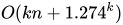
For example, there is an algorithm that solves the vertex cover problem in $O(kn+1.274^{k})$ time, where n is the number of vertices and k is the size of the vertex cover. This means that vertex cover is fixed-parameter tractable with the size of the solution as the parameter (its natural parameter). It is also possible to show vertex cover is in the parameterised version of Logspace, called logspace plus advice, parameterised problems solvable in space $O(\log |x|)+f(k)$.

Complexity classes

FPT

FPT (fixed parameter tractable) is the class of decision problems decidable in deterministic time $f(k)\cdot {|x|}^{O(1)}$, where f is a computable function. Typically, this function is thought of as single exponential, such as $2^{O(k)}$, but the definition admits functions that grow even faster. This is essential for a large part of the early history of this class. The crucial part of the definition is to exclude functions of the form $f(n,k)$, such as n^k or worse.

Strictly speaking this definition is what is called strongly uniform FPT. More general definitions allow for languages L where membership of (x,k) in L is decided by a machine M but f no longer has to be computable and this is called uniformly FPT, and finally L is called nonuniformly FPT if there is a series of algorithms M_k which decide membership in time $f(k)\cdot {|x|}^{O(1)}$. For most practical purposes, we can take $f(k)$ as being computable, but examples of uniform and nonuniform FPT problems have arisen from the Graph Minor Theorem.

The class FPL (fixed parameter linear) (or LFPT) is the class of problems solvable in time $f(k)\cdot |x|$ for some computable function f. FPL is thus a subclass of FPT. An example is the Boolean satisfiability problem, parameterised by the number of variables. A given formula of size m with k variables can be checked by brute force in time $O(2^{k}m)$. A vertex cover of size k in a graph of order n can be found in time $O(2^{k}n)$, so the vertex cover problem is also in FPL. Recent developments have identified the class TLFPT (true linear FPT) of problems solvable in time $c\cdot |x|+f(k)$ to be important. TLFPT does not equal LFPT by diagonalization. The model for both LFPT and TLFPT is the Word RAM model.

An example of a problem that is thought not to be in FPT is graph coloring parameterised by the number of colors. It is known that 3-coloring is NP-hard, and an algorithm for graph k-coloring in time $f(k)n^{O(1)}$ for $k=3$ would run in polynomial time in the size of the input. Thus, if graph coloring parameterised by the number of colors were in FPT, then P = NP.

There are a number of alternative definitions of FPT. For example, the running-time requirement can be replaced by $f(k)+|x|^{O(1)}$. Also, a parameterised problem is in FPT if it has a so-called kernel. Kernelization is a preprocessing technique that reduces the original instance to its "hard kernel", a possibly much smaller instance that is equivalent to the original instance but has a size that is bounded by a function in the parameter.

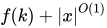
FPT is closed under a parameterised notion of reductions called fpt-reductions. We say that one parameterized problem $L$ fpt-reduces to $L'$ iff there exists two functions $(x,k)\mapsto x',k\mapsto k'$, such that

• $(x,k)\in L$ iff $(x',k')\in L'$
• $(x,k)\mapsto x'$ is itself fixed parameter tractable.
  • That is, there exists a constant $c$, and a function $k\mapsto k''$, such that $(x,k)\mapsto x'$ is computable in time $\leq k''|x|^{c}$

Obviously, FPT contains all polynomial-time computable problems. Moreover, it contains all optimisation problems in NP that allow an efficient polynomial-time approximation scheme (EPTAS). Here $k={\frac {1}{\epsilon }}$ is the parameter, and showing a PTAS is hard according to one of the hierarchies below (e.g. W[1]-hard) and this parameter implies that the problem. likely has no EPTAS, and hence no fully polynomial time approximatin scheme.

XP

XP is the class of parameterized problems that can be solved in time $n^{f(k)}$ for some computable function f.

These problems are called slicewise polynomial, in the sense that each "slice" of fixed k has a polynomial-time algorithm, although with a possibly different exponent for each k. Compare this with FPT, which merely allows a different constant prefactor for each value of k.

XP strictly contains FPT by diagonalization. There are some natural problems which are complete for XP such as determining winning strategies for the Pebble Game Problem for each parameter k.

para-NP is the class of decision problems decidable in nondeterministic time $f(k)\cdot |x|^{O(1)}$ for some computable function f.

${\textsf {FPT}}={\textsf {para-NP}}$ if and only if ${\textsf {P}}={\textsf {NP}}$.

A problem is para-NP-hard if it is ${\textsf {NP}}$-hard already for a constant value of the parameter. That is, there is a "slice" of fixed k that is ${\textsf {NP}}$-hard. A parameterized problem that is ${\textsf {para-NP}}$-hard cannot belong to the class ${\textsf {XP}}$, unless ${\textsf {P}}={\textsf {NP}}$. A classic example of a ${\textsf {para-NP}}$-hard parameterized problem is graph coloring, parameterized by the number k of colors, which is already ${\textsf {NP}}$-hard for $k=3$ (see Graph coloring § Computational complexity).

Hierarchies

In the parameterized complexity theory, there are some hierarchies of complexity classes. Each such class is closed under fpt-reduction. The most important ones are the W hierarchy and the A hierarchy.

Preliminary definitions

In general, there are two ways to define a complexity class: machine-theoretically and logically. In machine theory, a class is defined as the set of decision problems solvable by a class of machines. In logic, a class is defined as the set of decision problems definable by a class of logical formulas.

Boolean circuits

The Hamming weight (weight for short) of a binary string is the number of ones appearing in it.

A Boolean circuit is an acyclic directed graph where the nodes are one of the following gates: AND, OR, NOT. A small gate is a gate with fan-in 0, 1, or 2. Other gates are big. The weft is the largest number of big gates achievable on any path from an input to the output. The depth is the largest number of gates (small or big) achievable on any path from an input to the output. By definition, weft ≤ depth.

A Boolean circuit is monotone iff it uses no NOT gate. A Boolean circuit is antimonotone iff it is of the form $\phi (\neg x_{1},\dots ,\neg x_{n})$ where $x_{1},\dots ,x_{n}$ are all its inputs, and $\phi$ is monotone.

Finite model theory

Given any:

• ${\mathcal {L}}$, a first-order logical language with a finite set of relation symbols,
• $\Gamma$, a set of first-order logical formulas in that language,

we define $\operatorname {p-MC} (\Gamma )$ to be the parameterized model checking problem for this tuple. Each problem instance is:

• Input: $\phi \in \Gamma$, and a finite model $A$ for the language ${\mathcal {L}}$
• Parameter: $|\phi |$
• Output: Whether $A\models \phi$

A $\Sigma _{t}$ formula is of the form $\exists x_{1,1:m_{1}}\forall x_{2,1:m_{2}}\dots Qx_{t,1:m_{t}}\psi (x)$, such that the quantifiers are alternating between existence and for-all, and the formula inside $\psi (x)$ is quantifier-free (that is, written with just variables, Boolean connectives, and relations).

A $\Sigma _{t,s}$ formula is of the form $\exists x_{1,1:m_{1}}\forall x_{2,1:m_{2}}\dots Qx_{t,1:m_{t}}\psi (x)$, with the extra condition that $m_{2}\leq s,m_{3}\leq s,\dots ,m_{t}\leq s$.

Definition

Machine-theoretically, a parameterized problem is in the class W[w][d], if there is a fpt-reduction of the problem as follows:

• There exists constant integers $w,d$, such that
• every instance $(x,k)$ is transformed in fpt-time to a Boolean circuit that has weft at most w, and depth at most d,
• $(x,k)\in L$ if and only if the circuit has a satisfying assignment of weight k.

Here we see that "W" stands for "weight". Note that in the above definition, $w,d$ are independent of $(x,k)$, but the circuit itself depends on $(x,k)$, and may change if one changes either $x$ or $k$.

The class W[w] is then defined as their union:$$W[w][1]\subset W[w][2]\subset \dots \subset W[w]:=\bigcup _{d\geq 1}W[w][d]$$More succinctly, W[w] is the set of problems fpt-reducible to a family of instance-specific Boolean circuits with weft $\leq w$ and depth bounded by some problem-specific constant.

A normalized circuit of weft w and depth d is a circuit, where the first $d-w$ layers contain only small gates, and the last $w$ layers contain alternating big gates of AND and OR. One can iterate the associative laws and de Morgan distribution laws to normalize the circuit in fpt-time. Therefore, without loss of generality, we can consider only normalized circuits.

Model-theoretically, the class W[t] is defined as the class of problems fpt-reducible to $\operatorname {p-MC} (\Sigma _{t,1})$.

While the W hierarchy is a hierarchy contained in NP, the A hierarchy more closely mimics the polynomial-time hierarchy from classical complexity. Machine-theoretically, the A hierarchy of problems are defined as problems that are fpt-reducible to computations by certain kinds of alternating Turing machines. The "A" stands for "alternating".

Model-theoretically, the class A[t] is defined as the class of problems fpt-reducible to $\operatorname {p-MC} (\Sigma _{t})$.

For example, the k-clique problem can be specified as a model checking problem. The language has a single binary relation $E$, where $E(x,y)$ means "$x,y$ share an edge". Then, a finite model $A$ is a graph, and it has a k-clique iff $A\models \phi _{k}$, where$$\phi _{k}:=\exists x_{1:k},\bigwedge _{1\leq i<j\leq n}E(x_{i},x_{j})$$This shows that the k-clique problem is in $A[1]$.

A problem is A[i]-complete if it is A[i], and any A[i] problem fpt-reduces to it.

Basic properties

By definition,$$W[0]\subset W[1]\subset \cdots ,\quad W[i]\subset A[i],\quad A[0]\subset A[1]\subset \cdots$$${\mathsf {FPT}}=W[0]=A[0]$:

• $W[0]=A[0]$ since $\Sigma _{0}$ has no quantifiers at all, so there is no difference between $\Sigma _{0}$ and $\Sigma _{0,1}$.
• ${\mathsf {FPT}}\subset W[0]$. For any FPT problem $L$ can be trivially fpt-reduced thus: Solve the problem $(x,k)\in L$ in fpt-time, then output a trivial Yes/No circuit that does nothing except output the correct Boolean.
• ${\mathsf {FPT}}\supset W[0]$. For any W[0] problem $L$, and any problem-instance $c\in L$, the circuitry $c$ has 0 weft and $\leq d$ depth, where $d$ is fixed. Therefore, the output is determined by up to $2^{d}$ inputs. All other inputs are free for use. Therefore, one simply brute-force compute all $2^{2^{d}}$ possible inputs. If a certain input has weight k' and makes the circuit output True, then check if there are still enough inputs to fill the weight: $\#({\text{inputs of }}c)-2^{d}\geq k-k'$.

$W[1]=A[1]$.

W[1]

"W(1)" redirects here. For the mathematical constant, see omega constant.

Intuitively, problems in W[1] class can be interpreted of the form: Is there an object of size k with a certain locally-checkable property? In formula, it would be of the form $$\bigvee _{u_{1},\dots ,u_{k}}({\text{object constructed according to }}u_{1},\dots ,u_{k}{\text{ has a certain local property}})$$In fact, W[1] collapses to W[1, 2], the class of problems fpt-reducible to Boolean circuits of the form $\bigwedge _{i}(x_{i,1}\lor x_{i,2})$. That is, a big AND over many OR of fan-in 2.

Examples of W[1]-complete problems include:

• Independent set
  • Input: a graph G
  • Parameter: an integer k
  • Output: Whether G contains an independent set of size k
• Clique
  • Input: a graph G
  • Parameter: an integer k
  • Output: Whether G contains a clique of size k
• Bipartite nonblocker
  • Input: a bipartite graph $(V_{1},V_{2},E)$
  • Parameter: an integer k
  • Output: Whether there exists a subset $S\subset V_{1}$ of size k, such that any $v\in V_{2}$ has a neighbor $u\not \in S$. In other words, $S$ does not block $V_{2}$.
• Weight-k 2-satisfiability
  • Input: a conjunctive normal formula of form $\bigwedge _{i}(p_{i,1}\lor p_{i,2})$, where i ranges over clauses.
  • Parameter: an integer k
  • Output: Whether there exists a weight-k satisfying assignment to the formula.
• Short Turing machine problem.
  • Input: nondeterministic Turing machine M, a string x, an integer k.
  • Output: Whether there exists one computational path, with which M accepts x in at most k steps.

Note that the plain nonblocker problem is FPT.

Note on the nondeterministic Turing machine. The machine may be specified by one of any of the standard formulations. One usually considers the one-tape Turing machine, but the short Turing machine problem remains W[1] even if we allow with f(k) tapes and even f(k) of f(k)-dimensional tapes, but even with this extension, the restriction to f(k) tape alphabet size is FPT. Crucially, because the machine M itself is part of the problem input, the input size n is bigger than the number of states of M. In this way, the Turing machine can take one of $n$ possible computation paths per step, accessing $n^{O(k)}$ steps in total within time k. Thus, we see that W[1] is not obviously contained within FPT. Downey and Fellows argue that the Short Turing Machine problem is the natural analog of the Cook-Levin Theorem that the satisfiability problem is NP-complete and gives as compelling evidence that W[1] is not FPT as the Cook-Levin Theorem does that P does not equal NP.

The independent set problem can be encoded thus. Given each graph $(V,E)$, its independent set problem is encoded by the following weft-1 Boolean circuit:$$\Phi _{\text{IS}}(V,E):=\bigwedge _{\{u,v\}\in E}(\neg x_{u}\lor \neg x_{v})$$where $E$ is the set of edges in the graph. The graph has an independent set of size k iff there is a weight-k input to its Boolean circuit, such that it outputs 1.

The clique problem can be coded as $$\Phi _{\text{clique}}(V,E):=\bigwedge _{\{u,v\}\subset V,u\neq v,\{u,v\}\not \in E}(\neg x_{u}\lor \neg x_{v})$$It checks that any pair vertices that don't make an edge cannot be chosen, so any chosen set of vertices is forced to be a clique.

The short Turing machine problem can be converted to a Boolean formula using the same proof idea as of the Cook–Levin theorem, which shows SAT is NP-complete by coding Turing machine computational traces as Boolean formulas. The following proof is from. Specifically, define the propositional variables:

• $s_{t,i,j,a,b}$: at time t, the Turing machine is in state i, and transitions to state j, reading a, and writing b,
• $y_{t,p,a,b}$: at time t, the tape position p has symbol a, and at time (t+1) has symbol b.

Of the indices, time t and tape position p range over 1:k, The ranges of the indices to the Turing machine state i, j, transition m, and symbols a, b are determined by the description of the machine M, but they are both bounded within 1:n.

Then, the formula $\Phi _{{\text{STM}},k}(M,x)$ is a conjunction of clauses enforcing the following constraints:

• Every Turing machine state transition is not disallowed by the nondeterministic transition rule. These look like $s_{t,i,j,a,b}\to \neg s_{t+1,i',j',a',b'}$, in other words, $\neg s_{t,i,j,a,b}\lor \neg s_{t+1,i',j',a',b'}$. There are $O(kn^{4})$ such clauses.
• The Turing machine cannot be at two positions at a time, and cannot make two transitions at a time.
• Every tape cell state transition is not disallowed by the nondeterministic transition rule.
• Every tape cell state cannot have two symbols at a time.
• At time 0, the Turing machine is not out of its initial state and position, and x is not unwritten on the tape.
• The Turing machine is not in an unaccepting state at time k.

A computational trace through the Turing machine is then fully specified by setting k variables of $s_{t,i,j,a,b}$ to True to indicate the Turing machine state transitions at each time, and setting $k^{2}$ variables of $y_{t,p,a,b}$ to True to indicate the tape state transition at each time. This reduces the short Turing machine problem to a problem of finding a weight-$(k+k^{2})$ satisfying assignment to a weft-1, depth-2, antimonotone Boolean circuit.

One example showing how parameterised analysis differs from classical analysis is provided by Vapnik-Chervonenkis Dimension, which is known not to be NP-complete unless NP is a subset of DTIME$(n^{\log n})$ , and yet the parameterized version is W[1]-complete.

W[2]

W[2] problems are intuitively of the form: Guess an object of size k, perform some local processing on the object, then perform one global processing.

Examples of W[2]-complete problems include

• deciding if a given graph contains a dominating set of size k.
• deciding if a given nondeterministic multi-tape Turing machine accepts within k steps ("short multi-tape Turing machine acceptance" problem). Crucially, the branching is allowed to depend on n (like the W[1] variant), as is the number of tapes. An alternate W[2]-complete formulation allows only single-tape Turing machines, but the alphabet size may depend on n.

The dominating set problem has formula $\Psi _{\text{dom}}(V,E)=\bigwedge _{u\in V}\bigvee _{v\in \operatorname {Neighbor} [u]}x_{v}$.

W[i]

Some problems are known to be W[i]-complete, though they are in a computationally generic form, and are usually studied within parameterized complexity theory itself. Empirically, as of 2026, almost all naturally-occurring parameterized problems that they have studied, turned out to be W[0]-complete, W[1]-complete, or W[2]-complete. In this way it is similar to the Polynomial Hierarchy where few natural problems are at higher finite levels of the hierarchy. The following are usually used:

• Weighted i-Normalized Satisfiability: Given a Boolean formula, written as an AND of ORs of ANDs of ... of possibly negated variables, with $i+1$ layers of alternating ANDs or ORs, can it be satisfied by setting exactly k variables to 1?
  • Proof sketch: Any W[i]-circuit can be normalized in fpt-time by iterating association law and de Morgan distributive law, thus showing this problem is W[i]-complete.
• If i>0 is even, then
  • ${\text{monotone-}}W[i]=W[i]$.
  • Weighted Monotone i-Normalized Satisfiability is W[i]-complete.
  • Weighted Monotone (i+1)-Normalized Satisfiability is in W[i].
• If i>0 is odd, then
  • ${\text{antimonotone-}}W[i]=W[i]$
  • Weighted Antionotone i-Normalized Satisfiability is W[i]-complete.
  • If $i\geq 3$, then Weighted Antimonotone (i+1)-Normalized Satisfiability is in W[i].

These problems are essentially "artificial", in that they are not studied except within the context of parameterized complexity. The literature reports few naturally occurring problems that are W[i]-complete for $i\geq 3$:

• Detection of inclusion dependencies in relational databases is W[3]-complete.
• Certain problems in supply-chain models are W[3]-complete or W[4]-complete.

W[SAT]

W[SAT] is the class of problems fpt-reducible to weighted SAT problems:

• Input: a Boolean formula
• Parameter: k
• Output: Whether the formula has a weight-k satisfying assignment.

It contains all W[t].

W[P]

W[P] is the class of problems fpt-reducible to the problem of weighted Boolean circuit problems:

• Input: a Boolean circuit
• Parameter: k
• Output: Whether there exists a weight-k input such that the circuit outputs True.

It contains W[SAT], since a Boolean formula can be efficiently converted to a Boolean circuit. Note that the opposite is not true in general, since the equivalent Boolean formula to a Boolean circuit may be necessarily exponentially larger than the circuit.

Equivalently, it is the class of problems that can be decided by a nondeterministic $h(k)\cdot {|x|}^{O(1)}$-time Turing machine that makes at most $O(f(k)\cdot \log n)$ nondeterministic choices in the computation on $(x,k)$ (a k-restricted Turing machine).

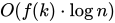
It is known that FPT is contained in W[P], and the inclusion is believed to be strict. However, proving that that inclusion is strict, would imply a solution to the P versus NP problem. It is possible that FPT coincides with W[P], and yet P is distinct from NP, but. this would imply much faster running times for NP problems then we currently believe.

Other connections to unparameterised computational complexity are that FPT equals W[P] if and only if circuit satisfiability can be decided in time $\exp(o(n))m^{O(1)}$, or if and only if there is a computable, nondecreasing, unbounded function f such that all languages recognised by a nondeterministic polynomial-time Turing machine using ⁠$f(n)\log n$⁠ nondeterministic choices are in P.

W[P] can be loosely thought of as the class of problems where we have a set S of n items, and we want to find a subset $T\subset S$ of size k such that a certain property holds. We can encode a choice as a list of k integers, stored in binary. Since the highest any of these numbers can be is n, $\lceil \log _{2}n\rceil$ bits are needed for each number. Therefore $k\cdot \lceil \log _{2}n\rceil$ total bits are needed to encode a choice. Therefore we can select a subset $T\subset S$ with $O(k\cdot \log n)$ nondeterministic choices.

Other classes

The W* hierarchy is similar to the W hierarchy, but it parameterizes depth, rather than holding it constant. The W*[t] class is defined as the class of problems fpt-reducible to this problem:

• Input: a Boolean circuit of weft at most t, and depth at most k,
• Parameter: k
• Output: Whether the Boolean circuit has a weight-k satisfying assignment.

It is related to W by:$$W^{*}[1]=W[1],\;W^{*}[2]=W[2],\;W[t]\subset W^{*}[t]\subset W[t+2],\quad \forall t\geq 1$$The AW hierarchy is obtained by adding alternation to the W hierarchy. The AW[t] class is defined as the class of problems fpt-reducible to this problem:

• Input: a Boolean circuit of weft at most t, and a partition of its inputs to $I_{1}\cup I_{2}\cup \cdots \cup I_{r}$
• Parameter: $(r,k_{1},\dots ,k_{r})$
• Output: Whether the Boolean circuit is satisfiable under alternating weight-$(k_{1},\dots ,k_{r})$ conditions.

The alternating weight-$(k_{1},\dots ,k_{r})$ is defined as follows:

• There exists a subset $J_{1}\subset I_{1}$ of size $k_{1}$, such that if we set exactly those inputs to True and the others to False, then,
• for any subset $J_{2}\subset I_{2}$ of size $k_{2}$, such that if we set exactly those inputs to True and the others to False, then,
• ...
• the Boolean circuit outputs True.

One can interpret this as a 2-player game, with the first player trying to make the circuit output True, and the second player trying to make the circuit output False. The first player makes a move by setting exactly $k_{1}$ inputs of $I_{1}$ to True and the others to False, then the second player makes a move on $I_{2}$, etc. The circuit is under alternating weight-$(k_{1},\dots ,k_{r})$ conditions iff player 1 has a winning strategy.

It turns out that the finite levels of this hierarchy collapses: $AW[1]=AW[2]=\cdots$. Thus, the literature writes just a common symbol for them: $AW[\ast ]:=AW[1]=AW[2]=\cdots$. Above this class remain two classes, AW[SAT] and AW[P], the first allows boolean formulas in the circuit and the second arbitrary ones. Notably, deciding if a nondeterministic Turing machine has an accepting computation visiting at most k tape squares is put hard for AW[SAT] and lies in AW[P].

Abrahamson, Downey and Fellows observe that many problem complete for PSPACE have parameterized versions in this class. For instance asking if an instance of the Generalised Geography problem has a k-move winning strategy is complete for this class.

There are a number of other hierarchies for parameterized complexity such as counting versions analogous to #P, as well as the M-hierarchy based around parameterizing the size of the problem rather than some aspect of the problem. For example, the problem of MiniCircuitSat_t takes inputs k and n in unary and a weft t circuit of size at most k log n, and asks if has a satisfying assignment. This problem is in FPT iff n variable 3 Sat is in DTIME(2^{o(n)}), that is, the Exponential Time Hypothesis fails. This observation allowed Cai and Juedes to give sharp lower bounds on parameterized exponential algorithms, assuming the ETH, and demonstrated a very close connection between parameterized complexity and subexponential complexity. Yijia Chen and Martin Grohe demonstrated that in fact there is an underlying isomorphism.

See also

• Parameterized approximation algorithm, for optimization problems an algorithm running in FPT time might approximate the solution.

References

• Chen, Jianer; Kanj, Iyad A.; Xia, Ge (2006). Improved Parameterized Upper Bounds for Vertex Cover. Mathematical Foundations of Computer Science. Vol. 4162. Berlin, Heidelberg: Springer. pp. 238–249. doi:10.1007/11821069_21. ISBN 978-3-540-37791-7.
• Fomin, Fedor V.; Lokshtanov, Daniel; Saurabh, Saket; Zehavi, Meirav (2019). Kernelization: Theory of Parameterized Preprocessing. Cambridge University Press. p. 528. doi:10.1017/9781107415157. ISBN 978-1-107-05776-0. S2CID 263888582.
• Gurevich, Yuri; Stockmeyer, Larry; Vishkin, Uzi (1984). Solving NP-hard problems on graphs that are almost trees and an application to facility location problems. Journal of the ACM. pp. 459–473.
• Grohe, Martin (1999). "Descriptive and Parameterized Complexity". Computer Science Logic. Lecture Notes in Computer Science. Vol. 1683. Springer Berlin Heidelberg. pp. 14–31. doi:10.1007/3-540-48168-0_3. ISBN 978-3-540-66536-6.
• The Computer Journal. Volume 51, Numbers 1 and 3 (2008). The Computer Journal. Special Double Issue on Parameterized Complexity with 15 survey articles, book review, and a Foreword by Guest Editors R. Downey, M. Fellows and M. Langston.

Textbooks

• Downey, Rod G.; Fellows, Michael R. (1999). Parameterized Complexity. Springer. doi:10.1007/978-1-4612-0515-9. ISBN 978-0-387-94883-6.
• Niedermeier, Rolf (2006). Invitation to Fixed-Parameter Algorithms. Oxford University Press. ISBN 978-0-19-856607-6. An introductory textbook.
• Flum, Jörg; Grohe, Martin (2006). Parameterized Complexity Theory. Springer. doi:10.1007/3-540-29953-X. ISBN 978-3-540-29952-3. An updated introduction to the 1999 textbook.
• Downey, Rodney G.; Fellows, Michael R. (2013). Fundamentals of Parameterized Complexity. Texts in Computer Science. London: Springer London. doi:10.1007/978-1-4471-5559-1. ISBN 978-1-4471-5558-4. A non-introductory textbook written to describe developments subsequent to the 1999 textbook.
• Cygan, Marek; Fomin, Fedor V.; Kowalik, Lukasz; Lokshtanov, Daniel; Marx, Daniel; Pilipczuk, Marcin; Pilipczuk, Michal; Saurabh, Saket (2015). Parameterized Algorithms. Springer. ISBN 978-3-319-21274-6.
• Chen, Hubie, Computability and Complexity, MIT Press, (2023). ISBN: 9780262048620. An undergraduate textbook with a chapter on parameterized complexity.
• Downey, Rodney G., Computability and Complexity: Fundamentals and Tools for Pursuing Scientific Applications, Springer, (2024) ISBN 978-3-031-53743-1. An undergraduate/beginning graduate textbook with a long chapter on parameterized complexity.

External links

• Wiki on parameterized complexity
• Compendium of Parameterized Problems
• https://complexityzoo.net/Complexity_Zoo:W