Massive fermion wave equation in Kerr spacetime
Chandrasekhar–Page equations describe the wave function of the spin-1/2 massive particles , that resulted by seeking a separable solution to the Dirac equation in Kerr metric or Kerr–Newman metric . In 1976, Subrahmanyan Chandrasekhar showed that a separable solution can be obtained from the Dirac equation in Kerr metric .[ 1] Don Page extended this work to Kerr–Newman metric , that is applicable to charged black holes.[ 2] Dirac equation in flat space-time in oblate spheroidal coordinates for the first time.
By assuming a normal mode decomposition of the form
e
i
(
m
ϕ
−
ω
t
)
{\displaystyle e^{i(m\phi -\omega t)}}
m
{\displaystyle m}
ω
{\displaystyle \omega }
(
r
,
θ
,
ϕ
)
{\displaystyle (r,\theta ,\phi )}
Dirac spinor components of the wave function,
[
F
1
(
r
,
θ
)
F
2
(
r
,
θ
)
G
1
(
r
,
θ
)
G
2
(
r
,
θ
)
]
e
i
(
m
ϕ
−
ω
t
)
{\displaystyle {\begin{bmatrix}F_{1}(r,\theta )\\F_{2}(r,\theta )\\G_{1}(r,\theta )\\G_{2}(r,\theta )\end{bmatrix}}e^{i(m\phi -\omega t)}}
can be expressed as product of radial and angular functions. The separation of variables is effected for the functions
f
1
=
(
r
−
i
a
cos
θ
)
F
1
{\displaystyle f_{1}=(r-ia\cos \theta )F_{1}}
f
2
=
(
r
−
i
a
cos
θ
)
F
2
{\displaystyle f_{2}=(r-ia\cos \theta )F_{2}}
g
1
=
(
r
+
i
a
cos
θ
)
G
1
{\displaystyle g_{1}=(r+ia\cos \theta )G_{1}}
g
2
=
(
r
+
i
a
cos
θ
)
G
2
{\displaystyle g_{2}=(r+ia\cos \theta )G_{2}}
a
{\displaystyle a}
angular momentum per unit mass of the black hole) as in
f
1
(
r
,
θ
)
=
R
−
(
r
)
S
−
(
θ
)
,
f
2
(
r
,
θ
)
=
R
+
(
r
)
S
+
(
θ
)
,
{\displaystyle f_{1}(r,\theta )=R_{-}(r)S_{-}(\theta ),\quad f_{2}(r,\theta )=R_{+}(r)S_{+}(\theta ),}
g
1
(
r
,
θ
)
=
R
+
(
r
)
S
−
(
θ
)
,
g
2
(
r
,
θ
)
=
R
−
(
r
)
S
+
(
θ
)
.
{\displaystyle g_{1}(r,\theta )=R_{+}(r)S_{-}(\theta ),\quad g_{2}(r,\theta )=R_{-}(r)S_{+}(\theta ).}
[ edit ] The angular functions satisfy the coupled eigenvalue equations,[ 3]
L
1
2
S
+
=
−
(
λ
−
a
μ
cos
θ
)
S
−
,
L
1
2
†
S
−
=
+
(
λ
+
a
μ
cos
θ
)
S
+
,
{\displaystyle {\begin{aligned}{\mathcal {L}}_{\frac {1}{2}}S_{+}&=-(\lambda -a\mu \cos \theta )S_{-},\\{\mathcal {L}}_{\frac {1}{2}}^{\dagger }S_{-}&=+(\lambda +a\mu \cos \theta )S_{+},\end{aligned}}}
where
μ
{\displaystyle \mu }
rest mass (measured in units so that it is the inverse of the Compton wavelength ), and
L
n
=
d
d
θ
+
(
m
csc
θ
−
a
ω
sin
θ
)
+
n
cot
θ
,
{\displaystyle {\mathcal {L}}_{n}={\frac {d}{{d}\theta }}+(m\csc \theta -a\omega \sin \theta )+n\cot \theta ,}
L
n
†
=
d
d
θ
−
(
m
csc
θ
−
a
ω
sin
θ
)
+
n
cot
θ
.
{\displaystyle {\mathcal {L}}_{n}^{\dagger }={\frac {d}{{d}\theta }}-(m\csc \theta -a\omega \sin \theta )+n\cot \theta .}
Eliminating
S
+
(
θ
)
{\displaystyle S_{+}(\theta )}
(
L
1
2
L
1
2
†
+
a
μ
sin
θ
λ
+
a
μ
cos
θ
L
1
2
†
+
λ
2
−
a
2
μ
2
cos
2
θ
)
S
−
=
0.
{\displaystyle \left({\mathcal {L}}_{\frac {1}{2}}{\mathcal {L}}_{\frac {1}{2}}^{\dagger }+{\frac {a\mu \sin \theta }{\lambda +a\mu \cos \theta }}{\mathcal {L}}_{\frac {1}{2}}^{\dagger }+\lambda ^{2}-a^{2}\mu ^{2}\cos ^{2}\theta \right)S_{-}=0.}
The function
S
+
{\displaystyle S_{+}}
adjoint equation , that can be obtained from the above equation by replacing
θ
{\displaystyle \theta }
π
−
θ
{\displaystyle \pi -\theta }
S
−
{\displaystyle S_{-}}
S
+
{\displaystyle S_{+}}
θ
=
0
{\displaystyle \theta =0}
θ
=
π
{\displaystyle \theta =\pi }
Properties and limiting solutions [ edit ] The eigenvalue problem depends on two continuous parameters, namely
a
ω
{\displaystyle a\omega }
a
μ
{\displaystyle a\mu }
a
ω
{\displaystyle a\omega }
a
μ
{\displaystyle a\mu }
j
=
1
/
2
,
3
/
2
,
…
{\displaystyle j=1/2,3/2,\dots }
m
=
−
j
,
−
j
+
1
,
…
,
j
−
1
,
j
{\displaystyle m=-j,-j+1,\dots ,j-1,j}
P
=
±
1.
{\displaystyle {\mathcal {P}}=\pm 1.}
[ 4]
S
±
=
s
=
±
1
2
S
j
,
m
,
P
(
a
ω
,
a
μ
)
,
λ
=
λ
j
,
m
,
P
(
a
ω
,
a
μ
)
.
{\displaystyle S_{\pm }={}_{s=\pm {\frac {1}{2}}}S_{j,m,{\mathcal {P}}}^{(a\omega ,a\mu )},\lambda =\lambda _{j,m,{\mathcal {P}}}^{(a\omega ,a\mu )}.}
The eigenvalue
λ
{\displaystyle \lambda }
square root of the generalised total anagular momentum squared.[ 5]
a
ω
>
0
,
a
μ
>
0
{\displaystyle a\omega >0,a\mu >0}
λ
j
,
m
,
P
(
a
ω
,
a
μ
)
=
−
λ
j
,
−
m
,
−
P
(
−
a
ω
,
a
μ
)
=
−
λ
j
,
m
,
−
P
(
a
ω
,
−
a
μ
)
=
λ
j
,
−
m
,
P
(
−
a
ω
,
−
a
μ
)
.
{\displaystyle \lambda _{j,m,{\mathcal {P}}}^{(a\omega ,a\mu )}=-\lambda _{j,-m,-{\mathcal {P}}}^{(-a\omega ,a\mu )}=-\lambda _{j,m,-{\mathcal {P}}}^{(a\omega ,-a\mu )}=\lambda _{j,-m,{\mathcal {P}}}^{(-a\omega ,-a\mu )}.}
Furthermore
s
S
j
,
m
,
P
(
a
ω
,
a
μ
)
(
θ
)
=
(
−
1
)
s
−
1
/
2
s
S
j
,
m
,
−
P
(
a
ω
,
−
a
μ
)
(
Θ
)
=
P
(
−
1
)
m
−
1
/
2
−
s
S
j
,
−
m
,
−
P
(
−
a
ω
,
a
μ
)
(
θ
)
=
P
(
−
1
)
j
+
m
−
s
S
j
,
m
,
P
(
a
ω
,
a
μ
)
(
π
−
θ
)
{\displaystyle {}_{s}S_{j,m,{\mathcal {P}}}^{(a\omega ,a\mu )}(\theta )=(-1)^{s-1/2}{}_{s}S_{j,m,-{\mathcal {P}}}^{(a\omega ,-a\mu )}(\Theta )={\mathcal {P}}(-1)^{m-1/2}{}_{-s}S_{j,-m,-{\mathcal {P}}}^{(-a\omega ,a\mu )}(\theta )={\mathcal {P}}(-1)^{j+m}{}_{-s}S_{j,m,{\mathcal {P}}}^{(a\omega ,a\mu )}(\pi -\theta )}
and the combinations thereof.
Non-rotating black hole (Schwarzschild black hole )
a
=
0
{\displaystyle a=0}
: The problem can be solved explicitly. The eigenvalues and eigenfunctions are given by
λ
j
,
m
,
P
(
0
,
0
)
=
P
(
j
+
1
/
2
)
,
{\displaystyle \lambda _{j,m,{\mathcal {P}}}^{(0,0)}={\mathcal {P}}(j+1/2),}
[
+
1
/
2
S
j
,
m
,
P
(
0
,
0
)
(
θ
)
−
1
/
2
S
j
,
m
,
P
(
0
,
0
)
(
θ
)
]
=
A
[
cos
θ
2
sin
θ
2
−
sin
θ
2
cos
θ
2
]
[
P
j
+
P
/
2
m
+
1
/
2
(
cos
θ
)
c
j
,
m
,
P
(
0
,
0
)
P
j
+
P
/
2
m
−
1
/
2
(
cos
θ
)
]
,
{\displaystyle {\begin{bmatrix}{}_{+1/2}S_{j,m,{\mathcal {P}}}^{(0,0)}(\theta )\\{}_{-1/2}S_{j,m,{\mathcal {P}}}^{(0,0)}(\theta )\end{bmatrix}}=A{\begin{bmatrix}\cos {\frac {\theta }{2}}&\sin {\frac {\theta }{2}}\\-\sin {\frac {\theta }{2}}&\cos {\frac {\theta }{2}}\end{bmatrix}}{\begin{bmatrix}P_{j+{\mathcal {P}}/2}^{m+1/2}(\cos \theta )\\c_{j,m,{\mathcal {P}}}^{(0,0)}P_{j+{\mathcal {P}}/2}^{m-1/2}(\cos \theta )\end{bmatrix}},}
where
P
{\displaystyle P}
associated Legendre polynomials and
c
j
,
m
,
P
(
0
,
0
)
=
P
(
j
+
P
/
2
+
1
/
2
)
−
m
,
A
=
(
j
−
m
)
!
2
π
(
j
+
m
)
!
.
{\displaystyle c_{j,m,{\mathcal {P}}}^{(0,0)}={\mathcal {P}}(j+{\mathcal {P}}/2+1/2)-m,\quad A={\sqrt {\frac {(j-m)!}{2\pi (j+m)!}}}.}
Special case
ω
=
±
μ
{\displaystyle \omega =\pm \mu }
: For the special case where
ω
=
+
μ
{\displaystyle \omega =+\mu }
[ 6]
λ
j
,
m
,
P
(
a
ω
,
a
ω
)
=
−
1
2
+
P
(
j
+
P
/
2
+
1
/
2
)
2
−
2
m
a
ω
+
a
2
ω
2
,
{\displaystyle \lambda _{j,m,{\mathcal {P}}}^{(a\omega ,a\omega )}=-{\frac {1}{2}}+{\mathcal {P}}{\sqrt {(j+{\mathcal {P}}/2+1/2)^{2}-2ma\omega +a^{2}\omega ^{2}}},}
[
+
1
/
2
S
j
,
m
,
P
(
0
,
0
)
(
θ
)
−
1
/
2
S
j
,
m
,
P
(
0
,
0
)
(
θ
)
]
=
A
[
cos
θ
2
sin
θ
2
−
sin
θ
2
cos
θ
2
]
[
P
j
+
P
/
2
m
+
1
/
2
(
cos
θ
)
c
j
,
m
,
P
(
a
ω
,
a
ω
)
P
j
+
P
/
2
m
−
1
/
2
(
cos
θ
)
]
,
{\displaystyle {\begin{bmatrix}{}_{+1/2}S_{j,m,{\mathcal {P}}}^{(0,0)}(\theta )\\{}_{-1/2}S_{j,m,{\mathcal {P}}}^{(0,0)}(\theta )\end{bmatrix}}=A{\begin{bmatrix}\cos {\frac {\theta }{2}}&\sin {\frac {\theta }{2}}\\-\sin {\frac {\theta }{2}}&\cos {\frac {\theta }{2}}\end{bmatrix}}{\begin{bmatrix}P_{j+{\mathcal {P}}/2}^{m+1/2}(\cos \theta )\\c_{j,m,{\mathcal {P}}}^{(a\omega ,a\omega )}P_{j+{\mathcal {P}}/2}^{m-1/2}(\cos \theta )\end{bmatrix}},}
where
c
j
,
m
,
P
(
a
ω
,
a
ω
)
=
[
(
j
+
P
/
2
+
1
/
2
)
2
−
m
2
]
/
(
λ
j
,
m
,
P
(
a
ω
,
a
ω
)
+
m
+
1
/
2
−
a
ω
)
,
{\displaystyle c_{j,m,{\mathcal {P}}}^{(a\omega ,a\omega )}=[(j+{\mathcal {P}}/2+1/2)^{2}-m^{2}]/(\lambda _{j,m,{\mathcal {P}}}^{(a\omega ,a\omega )}+m+1/2-a\omega ),}
A
=
(
j
+
P
/
2
+
1
/
2
)
2
π
(
j
+
P
/
2
−
m
−
1
/
2
)
!
(
j
+
P
/
2
+
m
+
1
/
2
)
!
(
1
+
P
(
m
−
a
ω
)
(
j
+
P
/
2
+
1
/
2
)
2
−
2
m
a
ω
+
a
2
ω
2
)
.
{\displaystyle A={\sqrt {{\frac {(j+{\mathcal {P}}/2+1/2)}{2\pi }}{\frac {(j+{\mathcal {P}}/2-m-1/2)!}{(j+{\mathcal {P}}/2+m+1/2)!}}\left(1+{\frac {{\mathcal {P}}(m-a\omega )}{\sqrt {(j+{\mathcal {P}}/2+1/2)^{2}-2ma\omega +a^{2}\omega ^{2}}}}\right)}}\,.}
When
ω
=
−
μ
{\displaystyle \omega =-\mu }
λ
j
,
m
,
P
(
a
ω
,
−
a
ω
)
=
1
2
+
P
(
j
+
P
/
2
+
1
/
2
)
2
−
2
m
a
ω
+
a
2
ω
2
,
{\displaystyle \lambda _{j,m,{\mathcal {P}}}^{(a\omega ,-a\omega )}={\frac {1}{2}}+{\mathcal {P}}{\sqrt {(j+{\mathcal {P}}/2+1/2)^{2}-2ma\omega +a^{2}\omega ^{2}}},}
[
+
1
/
2
S
j
,
m
,
P
(
a
ω
,
−
a
ω
)
(
θ
)
−
1
/
2
S
j
,
m
,
P
(
0
,
0
)
(
θ
)
]
=
A
[
cos
θ
2
−
sin
θ
2
sin
θ
2
cos
θ
2
]
[
P
j
+
P
/
2
m
+
1
/
2
(
cos
θ
)
c
j
,
m
,
P
(
a
ω
,
−
a
ω
)
P
j
+
P
/
2
m
−
1
/
2
(
cos
θ
)
]
,
{\displaystyle {\begin{bmatrix}{}_{+1/2}S_{j,m,{\mathcal {P}}}^{(a\omega ,-a\omega )}(\theta )\\{}_{-1/2}S_{j,m,{\mathcal {P}}}^{(0,0)}(\theta )\end{bmatrix}}=A{\begin{bmatrix}\cos {\frac {\theta }{2}}&-\sin {\frac {\theta }{2}}\\\sin {\frac {\theta }{2}}&\cos {\frac {\theta }{2}}\end{bmatrix}}{\begin{bmatrix}P_{j+{\mathcal {P}}/2}^{m+1/2}(\cos \theta )\\c_{j,m,{\mathcal {P}}}^{(a\omega ,-a\omega )}P_{j+{\mathcal {P}}/2}^{m-1/2}(\cos \theta )\end{bmatrix}},}
where
c
j
,
m
,
P
(
a
ω
,
−
a
ω
)
=
−
[
(
j
−
P
/
2
+
1
/
2
)
2
−
m
2
]
/
(
−
λ
j
,
m
,
P
(
a
ω
,
−
a
ω
)
+
m
+
1
/
2
−
a
ω
)
,
{\displaystyle c_{j,m,{\mathcal {P}}}^{(a\omega ,-a\omega )}=-[(j-{\mathcal {P}}/2+1/2)^{2}-m^{2}]/(-\lambda _{j,m,{\mathcal {P}}}^{(a\omega ,-a\omega )}+m+1/2-a\omega ),}
A
=
(
j
−
P
/
2
+
1
/
2
)
2
π
(
j
−
P
/
2
−
m
−
1
/
2
)
!
(
j
−
P
/
2
+
m
+
1
/
2
)
!
(
1
−
P
(
m
−
a
ω
)
(
j
−
P
/
2
+
1
/
2
)
2
−
2
m
a
ω
+
a
2
ω
2
)
.
{\displaystyle A={\sqrt {{\frac {(j-{\mathcal {P}}/2+1/2)}{2\pi }}{\frac {(j-{\mathcal {P}}/2-m-1/2)!}{(j-{\mathcal {P}}/2+m+1/2)!}}\left(1-{\frac {{\mathcal {P}}(m-a\omega )}{\sqrt {(j-{\mathcal {P}}/2+1/2)^{2}-2ma\omega +a^{2}\omega ^{2}}}}\right)}}\,.}
[ edit ] For convenience, let us write
σ
=
−
ω
.
{\displaystyle \sigma =-\omega .}
[ 3]
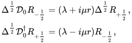
Δ
1
2
D
0
R
−
1
2
=
(
λ
+
i
μ
r
)
Δ
1
2
R
+
1
2
,
Δ
1
2
D
0
†
R
+
1
2
=
(
λ
−
i
μ
r
)
R
−
1
2
,
{\displaystyle {\begin{aligned}\Delta ^{\frac {1}{2}}{\mathcal {D}}_{0}R_{-{\frac {1}{2}}}&=(\lambda +i\mu r)\Delta ^{\frac {1}{2}}R_{+{\frac {1}{2}}},\\\Delta ^{\frac {1}{2}}{\mathcal {D}}_{0}^{\dagger }R_{+{\frac {1}{2}}}&=(\lambda -i\mu r)R_{-{\frac {1}{2}}},\end{aligned}}}
where
Δ
=
r
2
−
2
M
r
+
a
2
,
{\displaystyle \Delta =r^{2}-2Mr+a^{2},}
M
{\displaystyle M}
D
n
=
d
d
r
+
i
K
Δ
+
2
n
r
−
M
Δ
,
D
n
†
=
d
d
r
−
i
K
Δ
+
2
n
r
−
M
Δ
,
{\displaystyle {\mathcal {D}}_{n}={\frac {d}{{d}r}}+{\frac {iK}{\Delta }}+2n{\frac {r-M}{\Delta }},\quad {\mathcal {D}}_{n}^{\dagger }={\frac {d}{{d}r}}-{\frac {iK}{\Delta }}+2n{\frac {r-M}{\Delta }},}
and
K
=
(
r
2
+
a
2
)
σ
+
a
m
.
{\displaystyle K=(r^{2}+a^{2})\sigma +am.}
Δ
1
2
R
+
1
2
{\displaystyle \Delta ^{\frac {1}{2}}R_{+{\frac {1}{2}}}}
(
Δ
D
1
2
†
D
0
−
i
μ
Δ
λ
+
i
μ
r
D
0
−
λ
2
−
μ
2
r
2
)
R
−
1
2
=
0.
{\displaystyle \left(\Delta {\mathcal {D}}_{\frac {1}{2}}^{\dagger }{\mathcal {D}}_{0}-{\frac {i\mu \Delta }{\lambda +i\mu r}}{\mathcal {D}}_{0}-\lambda ^{2}-\mu ^{2}r^{2}\right)R_{-{\frac {1}{2}}}=0.}
The function
Δ
1
2
R
+
1
2
{\displaystyle \Delta ^{\frac {1}{2}}R_{+{\frac {1}{2}}}}
Reduction to one-dimensional scattering problem [ edit ] The problem of solving the radial functions for a particular eigenvalue of
λ
{\displaystyle \lambda }
Schrödinger equation ; see also Regge–Wheeler–Zerilli equations . Particularly, we end up with the equations
(
d
2
d
r
^
∗
2
+
σ
2
)
Z
±
=
V
±
Z
±
,
{\displaystyle \left({\frac {d^{2}}{d{\hat {r}}_{*}^{2}}}+\sigma ^{2}\right)Z^{\pm }=V^{\pm }Z^{\pm },}
where the Chandrasekhar–Page potentials
V
±
{\displaystyle V^{\pm }}
[ 3]
V
±
=
W
2
±
d
W
d
r
^
∗
,
W
=
Δ
1
2
(
λ
+
μ
2
r
2
)
3
/
2
ϖ
2
(
λ
2
+
μ
2
r
2
)
+
λ
μ
Δ
/
2
σ
,
{\displaystyle V^{\pm }=W^{2}\pm {\frac {dW}{d{\hat {r}}_{*}}},\quad W={\frac {\Delta ^{\frac {1}{2}}(\lambda +\mu ^{2}r^{2})^{3/2}}{\varpi ^{2}(\lambda ^{2}+\mu ^{2}r^{2})+\lambda \mu \Delta /2\sigma }},}
and
r
^
∗
=
r
∗
+
tan
−
1
(
μ
r
/
λ
)
/
2
σ
{\displaystyle {\hat {r}}_{*}=r_{*}+\tan ^{-1}(\mu r/\lambda )/2\sigma }
r
∗
=
r
+
2
M
ln
(
r
/
2
M
−
1
)
{\displaystyle r_{*}=r+2M\ln(r/2M-1)}
tortoise coordinate and
ϖ
2
=
r
2
+
a
2
+
a
m
/
σ
{\displaystyle \varpi ^{2}=r^{2}+a^{2}+am/\sigma }
Z
±
(
r
^
∗
)
{\displaystyle Z^{\pm }({\hat {r}}_{*})}
Z
±
=
ψ
+
±
ψ
−
{\displaystyle Z^{\pm }=\psi ^{+}\pm \psi ^{-}}
ψ
+
=
Δ
1
2
R
+
1
2
e
x
p
(
+
i
2
tan
−
1
μ
r
λ
)
,
ψ
−
=
R
−
1
2
e
x
p
(
−
i
2
tan
−
1
μ
r
λ
)
.
{\displaystyle \psi ^{+}=\Delta ^{\frac {1}{2}}R_{+{\frac {1}{2}}}\mathrm {exp} \left(+{\frac {i}{2}}\tan ^{-1}{\frac {\mu r}{\lambda }}\right),\quad \psi ^{-}=R_{-{\frac {1}{2}}}\mathrm {exp} \left(-{\frac {i}{2}}\tan ^{-1}{\frac {\mu r}{\lambda }}\right).}
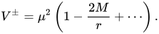
Unlike the Regge–Wheeler–Zerilli potentials , the Chandrasekhar–Page potentials do not vanish for
r
→
∞
{\displaystyle r\to \infty }
V
±
=
μ
2
(
1
−
2
M
r
+
⋯
)
.
{\displaystyle V^{\pm }=\mu ^{2}\left(1-{\frac {2M}{r}}+\cdots \right).}
As a result, the corresponding asymptotic behaviours for
Z
±
{\displaystyle Z^{\pm }}
r
→
∞
{\displaystyle r\to \infty }
Z
±
=
e
x
p
{
±
i
[
(
σ
2
−
μ
2
)
1
/
2
r
+
M
μ
2
(
σ
2
−
μ
2
)
1
/
2
ln
r
2
M
]
}
.
{\displaystyle Z^{\pm }=\mathrm {exp} \left\{\pm i\left[(\sigma ^{2}-\mu ^{2})^{1/2}r+{\frac {M\mu ^{2}}{(\sigma ^{2}-\mu ^{2})^{1/2}}}\ln {\frac {r}{2M}}\right]\right\}.}
↑ Chandrasekhar, S. (1976-06-29). "The solution of Dirac's equation in Kerr geometry". Proceedings of the Royal Society of London. Series A, Mathematical and Physical Sciences . 349 (1659). The Royal Society: 571– 575. Bibcode :1976RSPSA.349..571C . doi :10.1098/rspa.1976.0090 . ISSN 2053-9169 . S2CID 122791570 . ↑ Page, Don N. (1976-09-15). "Dirac equation around a charged, rotating black hole". Physical Review D . 14 (6). American Physical Society (APS): 1509– 1510. Bibcode :1976PhRvD..14.1509P . doi :10.1103/physrevd.14.1509 . ISSN 0556-2821 . 1 2 3 Chandrasekhar, S.,(1983). The mathematical theory of black holes. Clarenden Press, Section 104 ↑ Dolan, S. R., & Gair, J. R. (2009). The massive Dirac field on a rotating black hole spacetime: angular solutions. Classical and Quantum Gravity, 26(17), 175020. ↑ Batic, D., & Schmid, H. (2005). Chandrasekhar separation ansatz and the generalized total angular momentum for the Dirac equation in the Kerr-Newman metric. arXiv preprint gr-qc/0512112. ↑ Chakrabarti, S. K. (1984-01-09). "On mass-dependent spheroidal harmonics of spin one-half". Proceedings of the Royal Society of London. Series A, Mathematical and Physical Sciences . 391 (1800). The Royal Society: 27– 38. Bibcode :1984RSPSA.391...27C . doi :10.1098/rspa.1984.0002 . ISSN 2053-9169 . JSTOR 2397528 . S2CID 120673756 .








![{\displaystyle c_{j,m,{\mathcal {P}}}^{(a\omega ,a\omega )}=[(j+{\mathcal {P}}/2+1/2)^{2}-m^{2}]/(\lambda _{j,m,{\mathcal {P}}}^{(a\omega ,a\omega )}+m+1/2-a\omega ),}](https://wikimedia.org/api/rest_v1/media/math/render/svg/e79d6103be4581a0aaf31e0f6d54ee37d3647322)


![{\displaystyle c_{j,m,{\mathcal {P}}}^{(a\omega ,-a\omega )}=-[(j-{\mathcal {P}}/2+1/2)^{2}-m^{2}]/(-\lambda _{j,m,{\mathcal {P}}}^{(a\omega ,-a\omega )}+m+1/2-a\omega ),}](https://wikimedia.org/api/rest_v1/media/math/render/svg/2d132663307fd522b39079e9fa590686001910af)












![{\displaystyle Z^{\pm }=\mathrm {exp} \left\{\pm i\left[(\sigma ^{2}-\mu ^{2})^{1/2}r+{\frac {M\mu ^{2}}{(\sigma ^{2}-\mu ^{2})^{1/2}}}\ln {\frac {r}{2M}}\right]\right\}.}](https://wikimedia.org/api/rest_v1/media/math/render/svg/cb00acb5b14bbad412577c4a97cccfd7e11ff2bf)