Smith chart

For other uses, see Smith diagram (disambiguation).

"Volpert nomogram" redirects here. For other graphs attributed to Volpert, see Volpert graph (disambiguation).

(a) Sample Smith chart showing circles of constant $\operatorname {Re} (z)$ in red and arcs of constant $\operatorname {Im} (z)$ in blue.

(b) Animation illustrating the conformal mapping from the $z$-space, where constant-resistance and constant-reactance lines are straight, to the $\Gamma$-space, where they become circles and arcs. Pink lines denote $\operatorname {Re} (z)<0$, and black lines denote $\operatorname {Re} (z)\geq 0$.

The Smith chart is a circular nomogram used in radio frequency (RF) engineering to solve transmission line and impedance-matching problems. It plots a complex reflection coefficient ($\Gamma$) on a grid of normalized electrical impedance ($z$). Depending on the region, it is also known as the Smith diagram, Volpert–Smith chart, or Mizuhashi chart.

Because normalized impedance is complex, the chart maps two families of curves: circles of constant resistance ($\operatorname {Re} (z)$) and arcs of constant reactance ($\operatorname {Im} (z)$). Standard charts focus on passive circuits where resistance is non-negative ($\operatorname {Re} (z)\geq 0$). Regions outside the unit circle ($\operatorname {Re} (z)<0$) correspond to negative resistance, which is used for oscillator design and stability analysis.

The display allows engineers to evaluate multiple RF parameters at once, including admittance, $S_{nn}$ scattering parameters, noise figures, and stability boundaries.

Although paper charts have mostly been replaced by software for calculations, the display format remains standard across RF simulation software and vector network analyzers to visualize how parameters change with frequency.

History

The Smith chart emerged in the late 1930s through the independent work of Tōsaku Mizuhashi, Amiel R. Volpert, and Phillip H. Smith. It was initially known by several names before Smith chart became the standard name in the Western world by 1950.

Tōsaku Mizuhashi (水橋東作) independently proposed the chart in 1937, while Amiel R. Volpert (Амиэ́ль Р. Во́льперт) and Phillip H. Smith independently proposed it in 1939.

Smith initially developed a rectangular diagram, followed by a polar coordinate chart by 1936. With input from colleagues Enoch B. Ferrell and James W. McRae, who were familiar with conformal mapping, he refined it into its final form in early 1937. The chart was published in January 1939.

Smith originally called it the "transmission line chart". Early authors also used names such as "reflection chart", "circle diagram of impedance", "immittance chart", and "Z-plane chart". During the 1940s, researchers at MIT's Radiation Laboratory began referring to it simply as the "Smith chart". By 1950, the name had become the generally accepted term in the Western world.

Overview

The Smith chart converts normalized impedance into the complex reflection coefficient using a Möbius transformation. Impedances with positive real parts (passive loads) plot inside the unit circle, while those with negative real parts fall outside it.

A network analyzer displaying measured data on a Smith chart.

For an impedance chart, the transformation is:

$$\Gamma ={\frac {Z-Z_{0}}{Z+Z_{0}}}={\frac {z-1}{z+1}},$$

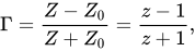
where $z=Z/Z_{0}$ is the complex impedance $Z$ normalized by the reference impedance $Z_{0}$.

Charts can show normalized impedance (Z chart), normalized admittance (Y chart), or both (YZ chart). On combined YZ charts, different colors distinguish the two grids.

The outer border has scales marked in wavelengths and degrees. The wavelength scale measures distance along a transmission line in distributed-element circuits, while the degree scale shows the phase angle of the reflection coefficient.

Because the chart uses normalized values, it applies to any system impedance. Its center represents the reference impedance (typically 50 Ω). To find the actual impedance or admittance, multiply the chart value by $Z_{0}$ or $Y_{0}$. Reflection coefficients are unitless and read directly off the chart.

Engineers use the chart for both distributed and lumped-element circuit analysis. For manual calculations, plotting a single point per frequency works well for narrowband applications (typically 5–10% bandwidth). Across wider bandwidths, connecting points from multiple frequencies forms a locus. This path shows how capacitive or inductive a load is, how difficult it is to match, and how well the component performs across the frequency range.

If a locus covers a wide impedance range, details can become hard to read, though specific regions can be enlarged for accuracy.

Mathematical basis

Basic use of an impedance Smith chart. A wave travels along a transmission line with characteristic impedance $Z_{0}$ toward a load with impedance $Z_{L}$ and normalized impedance $z=Z_{L}/Z_{0}$. The reflected wave has a reflection coefficient $\Gamma$, related to normalized impedance by $z=(1+\Gamma )/(1-\Gamma )$.

Normalization

A transmission line with characteristic impedance $Z_{0}$ has a characteristic admittance $Y_{0}=1/Z_{0}$. Any load impedance $Z$ or admittance $Y$ is normalized by dividing it by the corresponding characteristic value:

$$z={\frac {Z}{Z_{0}}},\quad y={\frac {Y}{Y_{0}}}={\frac {1}{z}}.$$

While impedance is measured in ohms (Ω) and admittance in siemens (S), dividing by $Z_{0}$ or $Y_{0}$ cancels these units. The resulting normalized values are dimensionless quantities, which are the only values plotted directly on a Smith chart.

Reflection coefficient and line propagation

Transmission lines terminated with an open circuit (top) and a short circuit (bottom). A pulse is completely reflected at both terminations, but the reflected voltage has opposite polarity in the two cases.

When a transmission line is terminated in a load impedance $Z_{L}$ that differs from its characteristic impedance $Z_{0}$, the incident (forward) wave $V_{\text{F}}$ and reflected wave $V_{\text{R}}$ superimpose to form a standing wave.

In complex phasor notation, measuring distance $\ell$ along the line from the load toward the generator gives:

$${\begin{aligned}V_{\text{F}}(\ell )&=Ae^{+\gamma \ell },\\V_{\text{R}}(\ell )&=Be^{-\gamma \ell },\end{aligned}}$$

where $A$ and $B$ are the complex voltage amplitudes at the load ($\ell =0$). The common time factor $e^{j\omega t}$ is suppressed assuming steady-state single-frequency operation.

The complex propagation constant is:

$$\gamma =\alpha +j\beta ,$$

where $\alpha$ is the attenuation constant and $\beta$ is the phase constant.

Variation along a line

As length $\ell$ of a lossless transmission line increases, input impedance traces a constant-SWR circle on the Smith chart.

The complex voltage reflection coefficient $\Gamma$ is the ratio of the reflected wave to the incident wave:

$$\Gamma ={\frac {V_{\text{R}}}{V_{\text{F}}}}={\frac {Be^{-\gamma \ell }}{Ae^{+\gamma \ell }}}=Ce^{-2\gamma \ell },$$

where $C$ is a constant.

For a uniform line with constant propagation constant $\gamma$, $\Gamma$ varies with position. On a lossy line ($\alpha >0$), this variation forms a spiral toward the center. On a lossless line ($\alpha =0$), attenuation is zero, simplifying the expression to:

$$\Gamma =\Gamma _{\text{L}}e^{-2j\beta \ell }=\Gamma _{\text{L}}\exp \left(-j{\frac {4\pi \ell }{\lambda }}\right),$$

where $\Gamma _{\text{L}}$ is the reflection coefficient at the load, $\ell$ is line length from the load, and $\lambda =2\pi /\beta$ is the line wavelength.

Because the angle changes by $2\pi$ radians over a distance of $\lambda /2$, the reflection coefficient and impedance repeat every half-wavelength. The outer scale of the Smith chart measures line length from $0$ to $0.5\,\lambda$.

Input impedance equation

If $V$ and $I$ are the total voltage and current at the termination, then:

$${\begin{aligned}V_{\text{F}}+V_{\text{R}}&=V,\\V_{\text{F}}-V_{\text{R}}&=Z_{0}I.\end{aligned}}$$

Dividing these equations gives the relationship between normalized load impedance $z$ and reflection coefficient $\Gamma$ (a Möbius transformation):

$$z={\frac {1+\Gamma }{1-\Gamma }}\quad \iff \quad \Gamma ={\frac {z-1}{z+1}}.$$

Because both $\Gamma$ and $z$ are dimensionless, frequency-dependent complex quantities, measurement values are plotted on a polar reflection diagram. Points inside the unit circle represent passive loads ($|\Gamma |\leq 1$).

Substituting $\Gamma (\ell )=\Gamma _{\text{L}}e^{-2j\beta \ell }$ into the impedance expression yields the standard transmission-line input equation:

$$Z_{\text{in}}=Z_{0}{\frac {Z_{\text{L}}+jZ_{0}\tan(\beta \ell )}{Z_{0}+jZ_{\text{L}}\tan(\beta \ell )}}.$$

On the Smith chart, this transformation corresponds to drawing a circle centered at the origin through $z$. Moving along the line corresponds to rotating along this circle using the outer wavelength scale.

Geometry of the Z chart

Chart regions

Angles on the chart are measured counterclockwise from the positive horizontal axis. The positive real axis extends from the center ($z=1$) to infinity ($z\to \infty$). The upper half-plane represents inductive impedances ($\operatorname {Im} (z)>0$), while the lower half-plane represents capacitive impedances ($\operatorname {Im} (z)<0$).

A perfectly matched load ($\Gamma =0$) sits at the center. Pure reactances lie on the outer boundary ($|\Gamma |=1$), with open and short circuits at extreme ends.

Constant resistance and reactance circles

Writing normalized impedance in terms of resistance and reactance as $z=r+jx$ gives:

$$\Gamma ={\frac {r^{2}+x^{2}-1}{(1+r)^{2}+x^{2}}}+j{\frac {2x}{(1+r)^{2}+x^{2}}}.$$

Plotting lines where $r$ or $x$ is constant forms two orthogonal families of circles on the complex plane. Standard charts plot these grid lines for passive conditions ($r\geq 0$).

Impedance–admittance conversion

Solving matching networks often requires converting between series elements (easiest in impedance $Z$) and parallel elements (easiest in admittance $Y$).

Converting a point between normalized impedance $z$ and normalized admittance $y=1/z$ corresponds to a 180° rotation around the origin at the same radius. For example, point ${\text{P}}_{1}$ ($z=0.80+j1.40$) rotates to diametrically opposite point ${\text{Q}}_{1}$ ($y=0.30-j0.54$).

Equivalent normalized impedance and admittance points

Normalized impedance ($z$)	Normalized admittance ($y=1/z$)
${\text{P}}_{1}=0.80+j1.40$	${\text{Q}}_{1}=0.30-j0.54$
${\text{P}}_{10}=0.10+j0.22$	${\text{Q}}_{10}=1.80-j3.90$

Reflection coefficient points on a Z chart and their 180° rotated equivalents on a Y chart.

Circuit elements and topology

Engineers choose between Z and Y charts based on circuit topology. Series components add directly as impedances ($Z_{\text{series}}=Z_{1}+Z_{2}+\dots$), while parallel components add directly as admittances ($Y_{\text{parallel}}=Y_{1}+Y_{2}+\dots$).

The normalized impedance and admittance for basic passive elements are:

$${\begin{aligned}{\text{Resistor:}}&\quad z={\frac {R}{Z_{0}}},&\quad y={\frac {G}{Y_{0}}}={\frac {Z_{0}}{R}}\\[0.5em]{\text{Inductor:}}&\quad z=j{\frac {\omega L}{Z_{0}}},&\quad y=-j{\frac {1}{\omega LY_{0}}}\\[0.5em]{\text{Capacitor:}}&\quad z=-j{\frac {1}{\omega CZ_{0}}},&\quad y=j{\frac {\omega C}{Y_{0}}}\end{aligned}}$$

where $Z_{0}=1/Y_{0}$ is the characteristic impedance.

Plotting examples

Example points plotted on a normalized impedance Smith chart.

A reflection coefficient of $0.63\angle 60^{\circ }$ plots at point ${\text{P}}_{1}$: 60° on the outer angle scale and at a radius of 0.63 from the center.

Examples of points plotted on the normalized impedance Smith chart

Point	Reflection coefficient (polar)	Normalized impedance (rectangular)
${\text{P}}_{1}$ (inductive)	$0.63\angle 60^{\circ }$	$0.80+j1.40$
${\text{P}}_{2}$ (inductive)	$0.73\angle 125^{\circ }$	$0.20+j0.50$
${\text{P}}_{3}$ (capacitive)	$0.44\angle -116^{\circ }$	$0.50-j0.50$

Applications

The Smith chart is used both for circuits whose dimensions are a significant fraction of a wavelength (distributed components) and for circuits much smaller than a wavelength (lumped elements). The boundary lies at roughly 5% of a wavelength at the operating frequency: above it, the electrical behavior of lumped components becomes unpredictable and distributed techniques are required. This is typical in microwave circuits, as well as shortwave, FM, and TV broadcasting where high power demands physically large components.

Distributed-component matching

For distributed components, the effect of moving along the transmission line on the reflection coefficient and impedance is accounted for using the outer circumferential scale of the Smith chart, which is calibrated in wavelengths.

The following example shows how a transmission line terminated with an arbitrary load can be matched at a single frequency using either a series or a parallel reactive component placed at a precise location.

Smith chart construction for distributed transmission-line matching.

Suppose a lossless air-spaced transmission line of characteristic impedance $Z_{0}=50\,\Omega$, operating at 800 MHz, is terminated with a circuit comprising a 17.5 Ω resistor in series with a 6.5 nH inductor. The reactance of the inductor at 800 MHz is:

$$j\omega L=j2\pi fL=j32.7\,\Omega ,$$

giving a total load impedance of:

$$Z_{\text{T}}=17.5+j32.7\,\Omega ,$$

and a normalized impedance of:

$$z_{\text{T}}={\frac {Z_{\text{T}}}{Z_{0}}}=0.35+j0.65.$$

This point is plotted on the Z Smith chart as ${\text{P}}_{20}$. Extending the line from the origin ${\text{O}}$ through ${\text{P}}_{20}$ to the outer wavelength scale intersects it at $L_{1}=0.098\lambda$. Because the line is lossless, a circle centered at the origin through ${\text{P}}_{20}$ represents the path of constant-magnitude reflection coefficient. At point ${\text{P}}_{21}$, this circle intersects the $r=1$ circle of constant normalized resistance at:

$$z_{{\text{P}}_{21}}=1.00+j1.52.$$

Extending the line ${\text{OP}}_{21}$ to the wavelength scale gives an intersection at $L_{2}=0.177\lambda$, making the distance from the termination:

$$L_{2}-L_{1}=0.177\lambda -0.098\lambda =0.079\lambda .$$

For an air-spaced transmission line, the wavelength at 800 MHz equals its free-space value:

$$\lambda ={\frac {c}{f}},$$

where $c$ is the speed of light and $f$ is frequency. This yields $\lambda =375\,{\text{mm}}$, placing the matching component 29.6 mm from the load.

The conjugate match for the impedance at ${\text{P}}_{21}$ is:

$$z_{\text{match}}=-j1.52.$$

Since the chart is in the normalized impedance plane, a series capacitor $C_{\text{m}}$ is required:

$$z_{\text{match}}=-j1.52=-{\frac {j}{\omega C_{\text{m}}Z_{0}}}=-{\frac {j}{2\pi fC_{\text{m}}Z_{0}}}.$$

Rearranging gives:

$$C_{\text{m}}={\frac {1}{1.52\,\omega Z_{0}}}={\frac {1}{1.52\times 2\pi fZ_{0}}},$$

which yields $C_{\text{m}}=2.6\,{\text{pF}}$. To match the load at 800 MHz, this capacitor is placed in series with the line 29.6 mm from the termination.

An alternative shunt match can be found by transforming the chart from normalized impedance to normalized admittance. Point ${\text{Q}}_{20}$ is the admittance equivalent of ${\text{P}}_{20}$; extending ${\text{OQ}}_{20}$ to the wavelength scale gives $L_{3}=0.152\lambda$. The nearest position toward the generator for a shunt conjugate match is ${\text{Q}}_{21}$ (at the same location as ${\text{P}}_{21}$, but representing admittance):

$$y_{{\text{Q}}_{21}}=1.00+j1.52.$$

The distance along the line for this shunt match is:

$$L_{2}+L_{3}=0.177\lambda +0.152\lambda =0.329\lambda ,$$

or 123 mm.

The conjugate matching component requires a normalized admittance of:

$$y_{\text{match}}=-j1.52.$$

A negative susceptance requires an inductor connected in parallel with the line. For an inductance $L_{\text{m}}$:

$$-j1.52=-{\frac {j}{\omega L_{\text{m}}Y_{0}}}=-{\frac {jZ_{0}}{2\pi fL_{\text{m}}}},$$

yielding $L_{\text{m}}=6.5\,{\text{nH}}$. A suitable shunt match is therefore a 6.5 nH inductor in parallel with the line, 123 mm from the load.

Lumped-element circuits

A lumped-element circuit that may be analyzed using a Smith chart.

For lumped-element circuits, movements on the chart are generated by the normalized impedances and admittances of individual components at the operating frequency. The outer wavelength scale is not used.

The circuit shown below is analyzed at an operating frequency of 100 MHz (wavelength $\lambda =3\,{\text{m}}$). It consists of two series capacitors and two shunt elements between the input and a load resistor. Because the component dimensions are on the order of millimeters, the lumped-element assumption holds. A reference impedance is still required for normalization; $Z_{0}=50\,\Omega$ is chosen because it equals the load resistance $R_{1}$.

Smith chart with graphical construction for analysis of the lumped circuit.

The analysis begins at the load and proceeds toward the input. Looking into $R_{1}$ alone, the normalized impedance is 1, represented by point ${\text{O}}$ at the chart center. Points in the Z plane are labeled ${\text{P}}$ and points in the Y plane are labeled ${\text{Q}}$; series elements are added in the Z plane and shunt elements in the Y plane. The table records the complete path around the chart, returning to the center and confirming a matched 50 Ω condition at the input.

Smith chart steps for analyzing the lumped-element circuit

Step	Plane	Normalized value ($x$ or $b$)	Component	Formula to solve	Result
${\text{O}}\to {\text{P}}_{1}$	Z	$-j0.80$	Series capacitor $C_{1}$	$-j0.80=-{\frac {j}{\omega C_{1}Z_{0}}}$	$C_{1}=40\,{\text{pF}}$
${\text{P}}_{1}\to {\text{Q}}_{1}$	Z → Y	Plane change at constant reflection coefficient
${\text{Q}}_{1}\to {\text{Q}}_{2}$	Y	$-j1.49$	Shunt inductor $L_{1}$	$-j1.49=-{\frac {j}{\omega L_{1}Y_{0}}}$	$L_{1}=53\,{\text{nH}}$
${\text{Q}}_{2}\to {\text{P}}_{2}$	Y → Z	Plane change at constant reflection coefficient
${\text{P}}_{2}\to {\text{P}}_{3}$	Z	$-j0.23$	Series capacitor $C_{2}$	$-j0.23=-{\frac {j}{\omega C_{2}Z_{0}}}$	$C_{2}=138\,{\text{pF}}$
${\text{P}}_{3}\to {\text{Q}}_{3}$	Z → Y	Plane change at constant reflection coefficient
${\text{Q}}_{3}\to {\text{O}}$	Y	$j1.14$	Shunt capacitor $C_{3}$	$j1.14={\frac {j\omega C_{3}}{Y_{0}}}$	$C_{3}=36\,{\text{pF}}$

Variations and extensions

Admittance chart

The Smith chart for admittance. Grid lines are rotated 180° about the center $\Gamma =0$.

The admittance (Y) Smith chart expresses the voltage reflection coefficient in terms of normalized admittance $y$ instead of impedance $z$. Because $y=1/z$:

$$y={\frac {1-\Gamma }{1+\Gamma }},\quad \Gamma ={\frac {1-y}{1+y}}.$$

The Y chart is identical to the Z chart, but rotated 180°. Writing $y=g+jb$ for conductance $g$ and susceptance $b$ gives:

$$\Gamma ={\frac {1-g^{2}-b^{2}}{(1+g)^{2}+b^{2}}}-j{\frac {2b}{(1+g)^{2}+b^{2}}}.$$

The region above the horizontal axis represents capacitive admittances ($b>0$), and the region below represents inductive admittances ($b<0$). A matched load ($\Gamma =0$) sits at the center, while pure reactances lie on the bounding unit circle ($|\Gamma |=1$).

Negative resistance

A Smith chart extended for negative resistance (${\text{Re}}(z)<0$).

The Smith chart can be extended for negative resistance (${\text{Re}}(z)<0$). In this region, $|\Gamma |>1$, meaning reflected power exceeds incident power. The extra power comes from an external DC source, as in an active amplifier.

Mapping onto a sphere

Smith chart projected onto a hemisphere

Constant resistance (${\text{Re}}(z)$)

Constant reactance (${\text{Im}}(z)$)

Combined grid lines

In 2011, Muller et al. proposed stereographically mapping the 2D reflection coefficient plane onto a 3D Riemann sphere. The resulting sphere has the following features:

See also

• Binary tiling
• Bode plot
• cis (mathematics)
• Circle diagram
• Nyquist plot
• Transversal (instrument making)

External links

• 3D Smith chart tool – interactive 2D and 3D Smith chart for active and passive circuits
• QuickSmith – open-source, web-based Smith chart educational tool
• Smith Chart Studio – interactive Smith Chart with dynamic high-DPI zoom, VSWR overlays, and real-time impedance matching trajectory simulation

References

[edit]- ↑ Ramo, Simon; Whinnery, John Roy; Van Duzer, Theodore (1965). Fields and Waves in Communications Electronics (1 ed.). John Wiley & Sons. pp. 35–39.
- ↑ Ramo, Simon; Whinnery, John Roy; Van Duzer, Theodore (1994). "5.9. The Smith Transmission-Line Chart / 5.10. Some Uses of the Smith Chart". Fields and Waves in Communications Electronics (3 ed.). John Wiley & Sons, Inc. pp. 236–245. ISBN 978-0-471-58551-0.
- ↑ Smith, Phillip Hagar (June 1969). Electronic Applications of the Smith Chart: In Waveguide, Circuit and Component Analysis (1 ed.). McGraw-Hill Book Company / Kay Electric Company. ISBN 0-07058930-5. LCCN 69-12411.
- 1 2 3 4 5 6 Smith, Phillip Hagar (October 2000) [1995]. Electronic Applications of the Smith Chart: In Waveguide, Circuit and Component Analysis (2 ed.). Noble Publishing Corporation. ISBN 1-884932-39-8. LCCN 00-045239. p. xiv:
[…] He was aware of the limitations and kept working on the problem until some time in 1936, when he developed a new diagram that eliminated most of the difficulties. The new chart was a special polar coordinate form in which all values of impedance components could be accommodated. […] Phil, however, suspected that a grid made up of a system of orthogonal circles might be more practical. With this in mind, he spoke to two of his co-workers, E.B. Ferrell and J.W. McRae. Because they were familiar with the principles of conformal mapping, they were able to develop the transformation whereby all data from zero to infinity could be accommodated. Fortunately, curves of constant standing wave ratio, constant attenuation and constant reflection coefficient were all circles coaxial with the center of the diagram. A diagram designed along these lines was constructed in early 1937. It was essentially the form still being used today.
- ↑ "Impedance Matching and Smith Chart Impedance" (Application note). Maxim Integrated Products, Inc. 2012 [2002-07-22]. Tutorial 742. Archived from the original on 2023-07-09. Retrieved 2023-07-09.
- ↑ Okamura [岡村], Fumiyoshi [史良] (August 1959). "Sumisuchāto wa nihonjin no dokusōde wanai ka" スミスチャートは日本人の独創ではないか ["Smith Chart" May Have Origin in Japan] (PDF). The Journal of the Institute of Electrical Communication Engineers of Japan [電気通信学会雑誌] (in Japanese). 1959 (8): 768–769. ISSN 0914-5273. Archived from the original (PDF) on 2017-11-16.
- ↑ Itō [伊藤], Ken'ichi [健一] (1999-11-01). Inpīdansu no hanashi インピーダンスのはなし [The story of impedance]. Science and Technology (in Japanese) (1 ed.). Nikkan Kogyo Shimbun. p. 26. ISBN 4-526-04463-6.
- ↑ Mori [森], Kunihiko [邦彦] (2013). "The Mizuhashi-Smith Chart". morikuni_net. Archived from the original on 2013-03-03. Retrieved 2023-06-24.
- 1 2 Kurochkin [Курочкин], Alexander Evdokimovich (2009). "Diagramma Vol'perta – Smita. Raschet i analiz kharakteristik usiliteley radiosignalov" Диаграмма Вольперта – Смита. Расчет и анализ характеристик усилителей радиосигналов [The Volpert–Smith diagram. Calculation and analysis of the characteristics of amplifiers of radio signals] (PDF) (in Russian). Minsk, Belarus: Belarusian State University of Informatics and Radio Electronics. ISBN 978-9-85-488-422-6. Archived (PDF) from the original on 2023-07-09. Retrieved 2023-07-09. p. 4: [In our country, a similar diagram is known as a circular nomogram of A. R. Volpert, who in 1939, independently of Smith developed and applied it to recalculate conductances and resistances in segments of transmission lines.]
{{cite web}}: CS1 maint: periodical has ISBN (link) - 1 2 Salov, Mikhail (March 2022). "4. Volpert–Smith Chart". Antenna Impedance Measurement and Matching (PDF) (Application note). Texas Instruments. p. 11. SWRA726. Archived (PDF) from the original on 2023-06-26. Retrieved 2023-06-26.
- 1 2 3 Gonzalez, Guillermo (1997). Microwave Transistor Amplifiers Analysis and Design (2 ed.). Prentice Hall. pp. 93–103. ISBN 0-13-254335-4.
- ↑ Pozar, David Michael (2005). Microwave Engineering (3 ed.). John Wiley & Sons, Inc. pp. 64–71. ISBN 0-471-44878-8.
- ↑ Bevelacqua, Peter Joseph (2013-01-11) [2010]. "The Smith Chart". Antenna-Theory.com. Archived from the original on 2023-07-08. Retrieved 2023-07-09.
- ↑ "Antenna Matching with a Vector Network Analyzer". Tektronix, Inc. 2017-10-06. Archived from the original on 2023-07-08. Retrieved 2023-07-09.
- 1 2 Linton, Jr., R. L. (January 1950). "Graph for Smith Chart" (PDF). Electronics. Vol. 23, no. 1. pp. 123, 158. ISSN 0013-5070. Retrieved 2023-07-22.
{{cite magazine}}: CS1 maint: url-status (link) - 1 2 "Impedance Measurement-Smith Chart with Example Plotted" (PDF). General Radio Experimenter. Vol. XXV, no. 6. Cambridge, Massachusetts, USA: General Radio Company. November 1950. pp. 5–7. Archived (PDF) from the original on 2023-07-22. Retrieved 2023-07-22.
- ↑ Mizuhashi [水橋], Tōsaku [東作] (December 1937). "Sì duānzǐ huílù no inpīdansu hensei to seigō kairo no riron" 四端子回路のインピーダンス変成と整合回路の理論 [Theory of Four-Terminals Impedance Transformation Circuit and Matching Circuit] (PDF). The Journal of the Institute of Electrical Communication Engineers of Japan [電気通信学会雑誌] (in Japanese). 1937 (12): 1053–1058. ISSN 0914-5273. Archived from the original (PDF) on 2017-11-16.
- ↑ Voltmer, David (2007-08-17). "8.2. The Smith Chart". In Balanis, Constantine A. (ed.). Fundamentals Of Electromagnetics 2. Quasistatics And Waves. Synthesis Lectures On Computational Electromagnetics. Vol. 2 (1 ed.). Morgan & Claypool. pp. 135–141. doi:10.2200/S00078ED1V01Y200612CEM015. ISBN 978-1-59829172-8. p. 135:
Though Volpert of the Soviet Union and Mizuhashi of Japan proposed essentially the same chart during the same year, Smith received the recognition.
- ↑ "Smith Chart". ETHW.org. 2018-02-26. Archived from the original on 2023-07-08. Retrieved 2021-03-30.
- ↑ Volpert [Во́льперт], Amiel Rafailovich [Амиэ́ль Рафаи́лович] [in Russian] (February 1940). "Nomogramma dlya rascheta dlinnykh liniy" Номограмма для расчета длинных линий [Nomogram for calculating long lines]. Производственно-технический бюллетень [Industrial and technical bulletin] (in Russian). Vol. 1940, no. 2. Leningrad, USSR. pp. 14–18.
- 1 2 3 4 Smith, Phillip Hagar (January 1939). "Transmission Line Calculator" (PDF). Electronics. Vol. 12, no. 1. pp. 29–31. ISSN 0013-5070. Archived (PDF) from the original on 2023-07-08. Retrieved 2023-07-09.
- 1 2 Smith, Phillip Hagar (January 1944). "An Improved Transmission Line Calculator" (PDF). Electronics. Vol. 17, no. 1. pp. 130–133, 318, 320, 322, 324–325. ISSN 0013-5070. Archived (PDF) from the original on 2023-01-31. Retrieved 2023-07-09.
- 1 2 3 Inan, Aziz S. (2005-07-03). Written at School of Engineering, University of Portland, Portland, Oregon, USA. Remembering Phillip H. Smith on his 100th Birthday (PDF). 2005 IEEE Antennas and Propagation Society International Symposium Digest. Vol. 3B. Washington, D.C., USA: IEEE Antennas and Propagation Society. pp. 129–132. doi:10.1109/APS.2005.1552450. eISSN 1947-1491. ISBN 0-7803-8883-6. ISSN 1522-3965. Archived (PDF) from the original on 2023-07-02. Retrieved 2023-07-02. (NB. This is a corrected version of the originally published paper.)
- ↑ Muller, Andrei A.; Soto Pacheco, Pablo; Dascălu, Dan [in Romanian]; Neculoiu, Dan; Boria, Vicente E. (2011). "A 3D Smith chart based on the Riemann sphere for active and passive microwave circuits". IEEE Microwave and Wireless Components Letters. 21 (6): 286–288. Bibcode:2011IMWCL..21..286M. doi:10.1109/LMWC.2011.2132697. hdl:10251/55107.
- Hayt, Jr., William Hart [at Wikidata] (1981). Engineering Electromagnetics (4 ed.). McGraw-Hill, Inc. pp. 428–433. ISBN 0-07-027395-2.
- Davidson, Colin William (1989). Transmission Lines for Communications with CAD Programs (2 ed.). Macmillan Education Ltd. pp. 80–85. ISBN 0-333-47398-1. Retrieved 2023-07-09.
- Muller, Andrei A.; Asavei, Victor; Moldoveanu, Alin; Sanabria-Codesal, Esther; Khadar, Riyaz A.; Popescu, Cornel; Dascălu, Dan [in Romanian]; Ionescu, Adrian M. (November 2020). "The 3D Smith Chart: From Theory to Experimental Reality". IEEE Microwave Magazine. 21 (11): 22–35. Bibcode:2020IMMag..21k..22M. doi:10.1109/MMM.2020.3014984.