Reduction of order

Reduction of order (or d’Alembert reduction) is a technique in mathematics for solving second-order linear ordinary differential equations. It is employed when one solution $y_{1}(x)$ is known and a second linearly independent solution $y_{2}(x)$ is desired. The method also applies to n-th order equations. In this case the ansatz will yield an (n−1)-th order equation for $v$.

Second-order linear ordinary differential equations

An example

Consider the general, homogeneous, second-order linear constant coefficient ordinary differential equation. (ODE) $$ay''(x)+by'(x)+cy(x)=0,$$ where $a,b,c$ are real non-zero coefficients. Two linearly independent solutions for this ODE can be straightforwardly found using characteristic equations except for the case when the discriminant, $b^{2}-4ac$, vanishes. In this case, $$ay''(x)+by'(x)+{\frac {b^{2}}{4a}}y(x)=0,$$ from which only one solution, $$y_{1}(x)=e^{-{\frac {b}{2a}}x},$$ can be found using its characteristic equation.

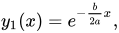
The method of reduction of order is used to obtain a second linearly independent solution to this differential equation using our one known solution. To find a second solution we take as a guess $$y_{2}(x)=v(x)y_{1}(x)$$ where $v(x)$ is an unknown function to be determined. Since $y_{2}(x)$ must satisfy the original ODE, we substitute it back in to get $$a\left(v''y_{1}+2v'y_{1}'+vy_{1}''\right)+b\left(v'y_{1}+vy_{1}'\right)+{\frac {b^{2}}{4a}}vy_{1}=0.$$ Rearranging this equation in terms of the derivatives of $v(x)$ we get $$\left(ay_{1}\right)v''+\left(2ay_{1}'+by_{1}\right)v'+\left(ay_{1}''+by_{1}'+{\frac {b^{2}}{4a}}y_{1}\right)v=0.$$

Since we know that $y_{1}(x)$ is a solution to the original problem, the coefficient of the last term is equal to zero. Furthermore, substituting $y_{1}(x)$ into the second term's coefficient yields (for that coefficient) $$2a\left(-{\frac {b}{2a}}e^{-{\frac {b}{2a}}x}\right)+be^{-{\frac {b}{2a}}x}=\left(-b+b\right)e^{-{\frac {b}{2a}}x}=0.$$

Therefore, we are left with $$ay_{1}v''=0.$$

Since $a$ is assumed non-zero and $y_{1}(x)$ is an exponential function (and thus always non-zero), we have $$v''=0.$$

This can be integrated twice to yield $$v(x)=c_{1}x+c_{2}$$ where $c_{1},c_{2}$ are constants of integration. We now can write our second solution as $$y_{2}(x)=(c_{1}x+c_{2})y_{1}(x)=c_{1}xy_{1}(x)+c_{2}y_{1}(x).$$

Since the second term in $y_{2}(x)$ is a scalar multiple of the first solution (and thus linearly dependent) we can drop that term, yielding a final solution of $$y_{2}(x)=xy_{1}(x)=xe^{-{\frac {b}{2a}}x}.$$

Finally, we can prove that the second solution $y_{2}(x)$ found via this method is linearly independent of the first solution by calculating the Wronskian $$W(y_{1},y_{2})(x)={\begin{vmatrix}y_{1}&xy_{1}\\y_{1}'&y_{1}+xy_{1}'\end{vmatrix}}=y_{1}(y_{1}+xy_{1}')-xy_{1}y_{1}'=y_{1}^{2}+xy_{1}y_{1}'-xy_{1}y_{1}'=y_{1}^{2}=e^{-{\frac {b}{a}}x}\neq 0.$$

Thus $y_{2}(x)$ is the second linearly independent solution we were looking for.

General method

Given the general non-homogeneous linear differential equation $$y''+p(t)y'+q(t)y=r(t)$$ and a single solution $y_{1}(t)$ of the homogeneous equation [$r(t)=0$], let us try a solution of the full non-homogeneous equation in the form: $$y_{2}=v(t)y_{1}(t)$$ where $v(t)$ is an arbitrary function. Thus $$y_{2}'=v'(t)y_{1}(t)+v(t)y_{1}'(t)$$ and $$y_{2}''=v''(t)y_{1}(t)+2v'(t)y_{1}'(t)+v(t)y_{1}''(t).$$

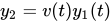
If these are substituted for $y$, $y'$, and $y''$ in the differential equation, then $$y_{1}(t)\,v''+(2y_{1}'(t)+p(t)y_{1}(t))\,v'+(y_{1}''(t)+p(t)y_{1}'(t)+q(t)y_{1}(t))\,v=r(t).$$

Since $y_{1}(t)$ is a solution of the original homogeneous differential equation, $y_{1}''(t)+p(t)y_{1}'(t)+q(t)y_{1}(t)=0$, so we can reduce to $$y_{1}(t)\,v''+(2y_{1}'(t)+p(t)y_{1}(t))\,v'=r(t)$$ which is a first-order differential equation for $v'(t)$ (reduction of order). Divide by $y_{1}(t)$, obtaining $$v''+\left({\frac {2y_{1}'(t)}{y_{1}(t)}}+p(t)\right)\,v'={\frac {r(t)}{y_{1}(t)}}.$$

One integrating factor is given by $\mu (t)=e^{\int ({\frac {2y_{1}'(t)}{y_{1}(t)}}+p(t))dt}$, and because

$\int \left({\frac {2y_{1}'(t)}{y_{1}(t)}}+p(t)\right)\,dt=2\int {\frac {y_{1}'(t)}{y_{1}(t)}}\,dt+\int p(t)\,dt=2\ln(y_{1}(t))+\int p(t)\,dt=\ln(y_{1}^{2}(t))+\int p(t)\,dt,$

this integrating factor can be more neatly expressed as $\mu (t)=e^{\ln(y_{1}^{2}(t))+\int p(t)\,dt}=y_{1}^{2}(t)e^{\int p(t)dt}.$ Multiplying the differential equation by the integrating factor $\mu (t)$, the equation for $v(t)$ can be reduced to $${\frac {d}{dt}}\left(v'(t)y_{1}^{2}(t)e^{\int p(t)dt}\right)=y_{1}(t)r(t)e^{\int p(t)dt}.$$

After integrating the last equation, $v'(t)$ is found, containing one constant of integration. Then, integrate $v'(t)$ to find the full solution of the original non-homogeneous second-order equation, exhibiting two constants of integration as it should: $$y_{2}(t)=v(t)y_{1}(t).$$

See also

• Variation of parameters

References

• Boyce, William E.; DiPrima, Richard C. (2005). Elementary Differential Equations and Boundary Value Problems (8th ed.). Hoboken, NJ: John Wiley & Sons, Inc. ISBN 978-0-471-43338-5.
• Teschl, Gerald (2012). Ordinary Differential Equations and Dynamical Systems. Providence: American Mathematical Society. ISBN 978-0-8218-8328-0.
• Eric W. Weisstein, Second-Order Ordinary Differential Equation Second Solution, From MathWorld—A Wolfram Web Resource.