Methods of matrix inversion

In linear algebra, the inverse square matrix $A$ is another square matrix $A^{-1}$ such that the product $A^{-1}A$ is the identity matrix. There are many methods for calculating an inverse matrix, if it exists.

Gaussian elimination

Gaussian elimination is a useful and easy way to compute the inverse of a matrix. To compute a matrix inverse using this method, an augmented matrix is first created with the left side being the matrix to invert and the right side being the identity matrix. Then, Gaussian elimination is used to convert the left side into the identity matrix, which causes the right side to become the inverse of the input matrix.

For example, take the following matrix: $$\mathbf {A} ={\begin{pmatrix}-1&{\tfrac {3}{2}}\\1&-1\end{pmatrix}}$$

The first step to compute its inverse is to create the augmented matrix $$\left(\!\!{\begin{array}{cc|cc}-1&{\tfrac {3}{2}}&1&0\\1&-1&0&1\end{array}}\!\!\right)$$

Call the first row of this matrix $R_{1}$ and the second row $R_{2}$. Then, add row 1 to row 2 $(R_{1}+R_{2}\to R_{2}).$ This yields $$\left(\!\!{\begin{array}{cc|cc}-1&{\tfrac {3}{2}}&1&0\\0&{\tfrac {1}{2}}&1&1\end{array}}\!\!\right)$$

Next, subtract row 2, multiplied by 3, from row 1 $(R_{1}-3\,R_{2}\to R_{1}),$ which yields $$\left(\!\!{\begin{array}{cc|cc}-1&0&-2&-3\\0&{\tfrac {1}{2}}&1&1\end{array}}\!\!\right)$$

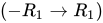
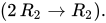
Finally, multiply row 1 by −1 $(-R_{1}\to R_{1})$ and row 2 by 2 $(2\,R_{2}\to R_{2}).$ This yields the identity matrix on the left side and the inverse matrix on the right:$$\left(\!\!{\begin{array}{cc|cc}1&0&2&3\\0&1&2&2\end{array}}\!\!\right)$$

Thus, $$\mathbf {A} ^{-1}={\begin{pmatrix}2&3\\2&2\end{pmatrix}}$$ It works because the process of Gaussian elimination can be viewed as a sequence of applying left matrix multiplication using elementary row operations using elementary matrices ($\mathbf {E} _{n}$), such as $\mathbf {E} _{n}\mathbf {E} _{n-1}\cdots \mathbf {E} _{2}\mathbf {E} _{1}\mathbf {A} =\mathbf {I}$

Applying right-multiplication using $\mathbf {A} ^{-1},$ we get $\mathbf {E} _{n}\mathbf {E} _{n-1}\cdots \mathbf {E} _{2}\mathbf {E} _{1}\mathbf {I} =\mathbf {I} \mathbf {A} ^{-1}.$ And the right side $\mathbf {I} \mathbf {A} ^{-1}=\mathbf {A} ^{-1},$ which is the inverse we want.

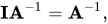
To obtain $\mathbf {E} _{n}\mathbf {E} _{n-1}\cdots \mathbf {E} _{2}\mathbf {E} _{1}\mathbf {I} ,$ we create the augmented matrix by combining A with I and applying Gaussian elimination. The two portions will be transformed using the same sequence of elementary row operations. When the left portion becomes I, the right portion applied the same elementary row operation sequence will become A⁻¹.

Newton's method

A generalization of Newton's method as used for a multiplicative inverse algorithm may be convenient if it is convenient to find a suitable starting seed:

$X_{k+1}=2X_{k}-X_{k}AX_{k}$

Victor Pan and John Reif have done work that includes ways of generating a starting seed.

Newton's method is particularly useful when dealing with families of related matrices that behave enough like the sequence manufactured for the homotopy above: sometimes a good starting point for refining an approximation for the new inverse can be the already obtained inverse of a previous matrix that nearly matches the current matrix. For example, the pair of sequences of inverse matrices used in obtaining matrix square roots by Denman–Beavers iteration. That may need more than one pass of the iteration at each new matrix, if they are not close enough together for just one to be enough. Newton's method is also useful for "touch up" corrections to the Gauss–Jordan algorithm which has been contaminated by small errors from imperfect computer arithmetic.

Cayley–Hamilton method

The Cayley–Hamilton theorem allows the inverse of A to be expressed in terms of det(A), traces and powers of A:

$\mathbf {A} ^{-1}={\frac {1}{\det(\mathbf {A} )}}\sum _{s=0}^{n-1}\mathbf {A} ^{s}\sum _{k_{1},k_{2},\ldots ,k_{n-1}}\prod _{l=1}^{n-1}{\frac {(-1)^{k_{l}+1}}{l^{k_{l}}k_{l}!}}\operatorname {tr} \left(\mathbf {A} ^{l}\right)^{k_{l}},$

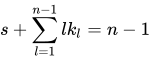
where n is size of A, and tr(A) is the trace of matrix A given by the sum of the main diagonal. The sum is taken over s and the sets of all $k_{l}\geq 0$ satisfying the linear Diophantine equation

$s+\sum _{l=1}^{n-1}lk_{l}=n-1$

The formula can be rewritten in terms of complete Bell polynomials of arguments $t_{l}=-(l-1)!\operatorname {tr} \left(A^{l}\right)$ as

$\mathbf {A} ^{-1}={\frac {1}{\det(\mathbf {A} )}}\sum _{s=1}^{n}\mathbf {A} ^{s-1}{\frac {(-1)^{n-1}}{(n-s)!}}B_{n-s}(t_{1},t_{2},\ldots ,t_{n-s})$

That is described in more detail under Cayley–Hamilton method.

Eigendecomposition

Main article: Eigendecomposition of a matrix

If matrix A can be eigendecomposed, and if none of its eigenvalues are zero, then A is invertible and its inverse is given by

$\mathbf {A} ^{-1}=\mathbf {Q} \mathbf {\Lambda } ^{-1}\mathbf {Q} ^{-1},$

where Q is the square (N × N) matrix whose ith column is the eigenvector $q_{i}$ of A, and Λ is the diagonal matrix whose diagonal entries are the corresponding eigenvalues, that is, $\Lambda _{ii}=\lambda _{i}.$ If A is symmetric, Q is guaranteed to be an orthogonal matrix, therefore $\mathbf {Q} ^{-1}=\mathbf {Q} ^{\mathrm {T} }.$ Furthermore, because Λ is a diagonal matrix, its inverse is easy to calculate:

$\left[\Lambda ^{-1}\right]_{ii}={\frac {1}{\lambda _{i}}}$

Cholesky decomposition

Main article: Cholesky decomposition

If matrix A is positive definite, then its inverse can be obtained as

$\mathbf {A} ^{-1}=\left(\mathbf {L} ^{*}\right)^{-1}\mathbf {L} ^{-1},$

where L is the lower triangular Cholesky decomposition of A, and L* denotes the conjugate transpose of L.

Solution using the adjugate

Main article: Cramer's rule

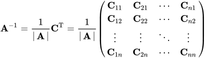
Writing the transpose of the matrix of cofactors, known as an adjugate matrix, may also be an efficient way to calculate the inverse of small matrices, but the recursive method is inefficient for large matrices. To determine the inverse, we calculate a matrix of cofactors:

$\mathbf {A} ^{-1}={1 \over {\begin{vmatrix}\mathbf {A} \end{vmatrix}}}\mathbf {C} ^{\mathrm {T} }={1 \over {\begin{vmatrix}\mathbf {A} \end{vmatrix}}}{\begin{pmatrix}\mathbf {C} _{11}&\mathbf {C} _{21}&\cdots &\mathbf {C} _{n1}\\\mathbf {C} _{12}&\mathbf {C} _{22}&\cdots &\mathbf {C} _{n2}\\\vdots &\vdots &\ddots &\vdots \\\mathbf {C} _{1n}&\mathbf {C} _{2n}&\cdots &\mathbf {C} _{nn}\\\end{pmatrix}}$

so that

$\left(\mathbf {A} ^{-1}\right)_{ij}={1 \over {\begin{vmatrix}\mathbf {A} \end{vmatrix}}}\left(\mathbf {C} ^{\mathrm {T} }\right)_{ij}={1 \over {\begin{vmatrix}\mathbf {A} \end{vmatrix}}}\left(\mathbf {C} _{ji}\right)$

where |A| is the determinant of A, C is the matrix of cofactors, and C^T represents the matrix transpose.

Inversion of 2 × 2 matrices

The cofactor equation listed above yields the following result for 2 × 2 matrices. Inversion of these matrices can be done as follows:

$\mathbf {A} ^{-1}={\begin{bmatrix}a&b\\c&d\\\end{bmatrix}}^{-1}={\frac {1}{\det \mathbf {A} }}{\begin{bmatrix}\,\,\,d&\!\!-b\\-c&\,a\\\end{bmatrix}}={\frac {1}{ad-bc}}{\begin{bmatrix}\,\,\,d&\!\!-b\\-c&\,a\\\end{bmatrix}}$

This is possible because 1/(ad − bc) is the reciprocal of the determinant of the matrix in question, and the same strategy could be used for other matrix sizes.

The Cayley–Hamilton method gives

$\mathbf {A} ^{-1}={\frac {1}{\det \mathbf {A} }}\left[\left(\operatorname {tr} \mathbf {A} \right)\mathbf {I} -\mathbf {A} \right]$

Inversion of 3 × 3 matrices

A computationally efficient 3 × 3 matrix inversion is given by

$\mathbf {A} ^{-1}={\begin{bmatrix}a&b&c\\d&e&f\\g&h&i\\\end{bmatrix}}^{-1}={\frac {1}{\det(\mathbf {A} )}}{\begin{bmatrix}\,A&\,B&\,C\\\,D&\,E&\,F\\\,G&\,H&\,I\\\end{bmatrix}}^{\mathrm {T} }={\frac {1}{\det(\mathbf {A} )}}{\begin{bmatrix}\,A&\,D&\,G\\\,B&\,E&\,H\\\,C&\,F&\,I\\\end{bmatrix}}$

(where the scalar A is not to be confused with the matrix A).

If the determinant is non-zero, the matrix is invertible, with the entries of the intermediary matrix on the right side above given by

${\begin{alignedat}{6}A&={}&(ei-fh),&\quad &D&={}&-(bi-ch),&\quad &G&={}&(bf-ce),\\B&={}&-(di-fg),&\quad &E&={}&(ai-cg),&\quad &H&={}&-(af-cd),\\C&={}&(dh-eg),&\quad &F&={}&-(ah-bg),&\quad &I&={}&(ae-bd).\\\end{alignedat}}$

The determinant of A can be computed by applying the rule of Sarrus as follows:

$\det(\mathbf {A} )=aA+bB+cC$

The Cayley–Hamilton decomposition gives

$\mathbf {A} ^{-1}={\frac {1}{\det(\mathbf {A} )}}\left({\tfrac {1}{2}}\left[(\operatorname {tr} \mathbf {A} )^{2}-\operatorname {tr} (\mathbf {A} ^{2})\right]\mathbf {I} -\mathbf {A} \operatorname {tr} \mathbf {A} +\mathbf {A} ^{2}\right)$

The general 3 × 3 inverse can be expressed concisely in terms of the cross product and triple product. If a matrix $\mathbf {A} ={\begin{bmatrix}\mathbf {x} _{0}&\mathbf {x} _{1}&\mathbf {x} _{2}\end{bmatrix}}$ (consisting of three column vectors, $\mathbf {x} _{0}$, $\mathbf {x} _{1}$, and $\mathbf {x} _{2}$) is invertible, its inverse is given by

$\mathbf {A} ^{-1}={\frac {1}{\det(\mathbf {A} )}}{\begin{bmatrix}{(\mathbf {x} _{1}\times \mathbf {x} _{2})}^{\mathrm {T} }\\{(\mathbf {x} _{2}\times \mathbf {x} _{0})}^{\mathrm {T} }\\{(\mathbf {x} _{0}\times \mathbf {x} _{1})}^{\mathrm {T} }\end{bmatrix}}$

The determinant of A, det(A), is equal to the triple product of x₀, x₁, and x₂—the volume of the parallelepiped formed by the rows or columns:

$\det(\mathbf {A} )=\mathbf {x} _{0}\cdot (\mathbf {x} _{1}\times \mathbf {x} _{2})$

The correctness of the formula can be checked by using cross- and triple-product properties and by noting that for groups, left and right inverses always coincide. Intuitively, because of the cross products, each row of A^–1 is orthogonal to the non-corresponding two columns of A (causing the off-diagonal terms of $\mathbf {I} =\mathbf {A} ^{-1}\mathbf {A}$ be zero). Dividing by

$\det(\mathbf {A} )=\mathbf {x} _{0}\cdot (\mathbf {x} _{1}\times \mathbf {x} _{2})$

causes the diagonal entries of I = A⁻¹A to be unity. For example, the first diagonal is:

$1={\frac {1}{\mathbf {x_{0}} \cdot (\mathbf {x} _{1}\times \mathbf {x} _{2})}}\mathbf {x_{0}} \cdot (\mathbf {x} _{1}\times \mathbf {x} _{2})$

Inversion of 4 × 4 matrices

With increasing dimension, expressions for the inverse of A get complicated. For n = 4, the Cayley–Hamilton method leads to an expression that is still tractable:

${\begin{aligned}\mathbf {A} ^{-1}={\frac {1}{\det(\mathbf {A} )}}{\Bigl (}&{\tfrac {1}{6}}{\bigl (}(\operatorname {tr} \mathbf {A} )^{3}-3\operatorname {tr} \mathbf {A} \operatorname {tr} (\mathbf {A} ^{2})+2\operatorname {tr} (\mathbf {A} ^{3}){\bigr )}\mathbf {I} \\[-3mu]&\ \ \ -{\tfrac {1}{2}}\mathbf {A} {\bigl (}(\operatorname {tr} \mathbf {A} )^{2}-\operatorname {tr} (\mathbf {A} ^{2}){\bigr )}+\mathbf {A} ^{2}\operatorname {tr} \mathbf {A} -\mathbf {A} ^{3}{\Bigr )}\end{aligned}}$

Blockwise inversion

Let

$\mathbf {M} ={\begin{bmatrix}\mathbf {A} &\mathbf {B} \\\mathbf {C} &\mathbf {D} \end{bmatrix}}$

where A, B, C and D are matrix sub-blocks of arbitrary size and $\mathbf {M} /\mathbf {A$ :=\mathbf {D} -\mathbf {C} \mathbf {A} ^{-1}\mathbf {B} } is the Schur complement of A. (A must be square, so that it can be inverted. Furthermore, A and D − CA⁻¹B must be nonsingular.)

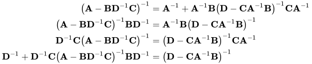
Matrices can also be inverted blockwise by using the analytic inversion formula:

${\begin{bmatrix}\mathbf {A} &\mathbf {B} \\\mathbf {C} &\mathbf {D} \end{bmatrix}}^{-1}={\begin{bmatrix}\mathbf {A} ^{-1}+\mathbf {A} ^{-1}\mathbf {B} \ (\mathbf {M} /\mathbf {A} )^{-1}\mathbf {CA} ^{-1}&-\mathbf {A} ^{-1}\mathbf {B} \left(\mathbf {M} /\mathbf {A} \right)^{-1}\\-\left(\mathbf {M} /\mathbf {A} \right)^{-1}\mathbf {CA} ^{-1}&\left(\mathbf {M} /\mathbf {A} \right)^{-1}\end{bmatrix}},$ 1

The strategy is particularly advantageous if A is diagonal and M / A is a small matrix, since they are the only matrices requiring inversion.

The nullity theorem says that the nullity of A equals the nullity of the sub-block in the lower right of the inverse matrix, and that the nullity of B equals the nullity of the sub-block in the upper right of the inverse matrix.

The inversion procedure that led to Equation (1) performed matrix block operations that operated on C and D first. Instead, if A and B are operated on first, and provided D and M / D := A − BD⁻¹C are nonsingular, the result is

${\begin{bmatrix}\mathbf {A} &\mathbf {B} \\\mathbf {C} &\mathbf {D} \end{bmatrix}}^{-1}={\begin{bmatrix}\left(\mathbf {M} /\mathbf {D} \right)^{-1}&-\left(\mathbf {M} /\mathbf {D} \right)^{-1}\mathbf {BD} ^{-1}\\-\mathbf {D} ^{-1}\mathbf {C} \left(\mathbf {M} /\mathbf {D} \right)^{-1}&\quad \mathbf {D} ^{-1}+\mathbf {D} ^{-1}\mathbf {C} \left(\mathbf {M} /\mathbf {D} \right)^{-1}\mathbf {BD} ^{-1}\end{bmatrix}}.$ 2

Equating the upper-left sub-matrices of Equations (1) and (2) leads to

${\begin{aligned}\left(\mathbf {A} -\mathbf {BD} ^{-1}\mathbf {C} \right)^{-1}&=\mathbf {A} ^{-1}+\mathbf {A} ^{-1}\mathbf {B} \left(\mathbf {D} -\mathbf {CA} ^{-1}\mathbf {B} \right)^{-1}\mathbf {CA} ^{-1}\\\left(\mathbf {A} -\mathbf {BD} ^{-1}\mathbf {C} \right)^{-1}\mathbf {BD} ^{-1}&=\mathbf {A} ^{-1}\mathbf {B} \left(\mathbf {D} -\mathbf {CA} ^{-1}\mathbf {B} \right)^{-1}\\\mathbf {D} ^{-1}\mathbf {C} \left(\mathbf {A} -\mathbf {BD} ^{-1}\mathbf {C} \right)^{-1}&=\left(\mathbf {D} -\mathbf {CA} ^{-1}\mathbf {B} \right)^{-1}\mathbf {CA} ^{-1}\\\mathbf {D} ^{-1}+\mathbf {D} ^{-1}\mathbf {C} \left(\mathbf {A} -\mathbf {BD} ^{-1}\mathbf {C} \right)^{-1}\mathbf {BD} ^{-1}&=\left(\mathbf {D} -\mathbf {CA} ^{-1}\mathbf {B} \right)^{-1}\end{aligned}}$ 3

where Equation (3) is the Woodbury matrix identity, which is equivalent to the binomial inverse theorem.

If A and D are both invertible, then the above two block matrix inverses can be combined to provide the simple factorization

${\begin{bmatrix}\mathbf {A} &\mathbf {B} \\\mathbf {C} &\mathbf {D} \end{bmatrix}}^{-1}={\begin{bmatrix}\left(\mathbf {A} -\mathbf {B} \mathbf {D} ^{-1}\mathbf {C} \right)^{-1}&\mathbf {0} \\\mathbf {0} &\left(\mathbf {D} -\mathbf {C} \mathbf {A} ^{-1}\mathbf {B} \right)^{-1}\end{bmatrix}}{\begin{bmatrix}\mathbf {I} &-\mathbf {B} \mathbf {D} ^{-1}\\-\mathbf {C} \mathbf {A} ^{-1}&\mathbf {I} \end{bmatrix}}.$ 2

By the Weinstein–Aronszajn identity, one of the two matrices in the block-diagonal matrix is invertible exactly when the other is.

This formula simplifies significantly when the upper right block matrix B is the zero matrix. This formulation is useful when the matrices A and D have relatively simple inverse formulas (or pseudo inverses in the case where the blocks are not all square. In this special case, the block matrix inversion formula stated in full generality above becomes

${\begin{bmatrix}\mathbf {A} &\mathbf {0} \\\mathbf {C} &\mathbf {D} \end{bmatrix}}^{-1}={\begin{bmatrix}\mathbf {A} ^{-1}&\mathbf {0} \\-\mathbf {D} ^{-1}\mathbf {CA} ^{-1}&\mathbf {D} ^{-1}\end{bmatrix}}$

If the given invertible matrix is a symmetric matrix with invertible block A the following block inverse formula holds

${\begin{bmatrix}\mathbf {A} &\mathbf {C} ^{T}\\\mathbf {C} &\mathbf {D} \end{bmatrix}}^{-1}={\begin{bmatrix}\mathbf {A} ^{-1}+\mathbf {A} ^{-1}\mathbf {C} ^{T}\mathbf {S} ^{-1}\mathbf {C} \mathbf {A} ^{-1}&-\mathbf {A} ^{-1}\mathbf {C} ^{T}\mathbf {S} ^{-1}\\-\mathbf {S} ^{-1}\mathbf {C} \mathbf {A} ^{-1}&\mathbf {S} ^{-1}\end{bmatrix}},$ 4

where $\mathbf {S} =\mathbf {D} -\mathbf {C} \mathbf {A} ^{-1}\mathbf {C} ^{T}$. This requires 2 inversions of the half-sized matrices A and S and only 4 multiplications of half-sized matrices, if organized properly $${\begin{aligned}\mathbf {W} _{1}&=\mathbf {C} \mathbf {A} ^{-1},\\[3mu]\mathbf {W} _{2}&=\mathbf {W} _{1}\mathbf {C} ^{T}=\mathbf {C} \mathbf {A} ^{-1}\mathbf {C} ^{T},\\[3mu]\mathbf {W} _{3}&=\mathbf {S} ^{-1}\mathbf {W} _{1}=\mathbf {S} ^{-1}\mathbf {C} \mathbf {A} ^{-1},\\[3mu]\mathbf {W} _{4}&=\mathbf {W} _{1}^{T}\mathbf {W} _{3}=\mathbf {A} ^{-1}\mathbf {C} ^{T}\mathbf {S} ^{-1}\mathbf {C} \mathbf {A} ^{-1},\end{aligned}}$$ together with some additions, subtractions, negations and transpositions of negligible complexity. Any matrix $\mathbf {M}$ has an associated positive semidefinite, symmetric matrix $\mathbf {M} ^{T}\mathbf {M}$, which is exactly invertible (and positive definite), if and only if $\mathbf {M}$ is invertible. By writing $\mathbf {M} ^{-1}=\left(\mathbf {M} ^{T}\mathbf {M} \right)^{-1}\mathbf {M} ^{T}$ matrix inversion can be reduced to inverting symmetric matrices and 2 additional matrix multiplications, because the positive definite matrix $\mathbf {M} ^{T}\mathbf {M}$ satisfies the invertibility condition for its left upper block A.

Those formulas together allow to construct a divide and conquer algorithm that uses blockwise inversion of associated symmetric matrices to invert a matrix with the same time complexity as the matrix multiplication algorithm that is used internally. Research into matrix multiplication complexity shows that there exist matrix multiplication algorithms with a complexity of O(n^2.371552) operations, while the best proven lower bound is Ω(n² log n).

By Neumann series

If a matrix A has the property that

$\lim _{n\to \infty }(\mathbf {I} -\mathbf {A} )^{n}=0$

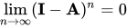
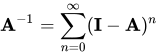
then A is nonsingular and its inverse may be expressed by a Neumann series:

$\mathbf {A} ^{-1}=\sum _{n=0}^{\infty }(\mathbf {I} -\mathbf {A} )^{n}$

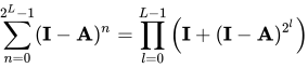
Truncating the sum results in an "approximate" inverse which may be useful as a preconditioner. Note that a truncated series can be accelerated exponentially by noting that the Neumann series is a geometric sum. As such, it satisfies

$\sum _{n=0}^{2^{L}-1}(\mathbf {I} -\mathbf {A} )^{n}=\prod _{l=0}^{L-1}\left(\mathbf {I} +(\mathbf {I} -\mathbf {A} )^{2^{l}}\right)$

Therefore, only 2L − 2 matrix multiplications are needed to compute 2^L terms of the sum.

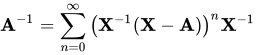
More generally, if A is "near" the invertible matrix X in the sense that

$\lim _{n\to \infty }\left(\mathbf {I} -\mathbf {X} ^{-1}\mathbf {A} \right)^{n}=0\mathrm {~~or~~} \lim _{n\to \infty }\left(\mathbf {I} -\mathbf {A} \mathbf {X} ^{-1}\right)^{n}=0$

then A is nonsingular and its inverse is

$\mathbf {A} ^{-1}=\sum _{n=0}^{\infty }\left(\mathbf {X} ^{-1}(\mathbf {X} -\mathbf {A} )\right)^{n}\mathbf {X} ^{-1}~$

If it is also the case that A − X has rank 1 then this simplifies to

$\mathbf {A} ^{-1}=\mathbf {X} ^{-1}-{\frac {\mathbf {X} ^{-1}(\mathbf {A} -\mathbf {X} )\mathbf {X} ^{-1}}{1+\operatorname {tr} \left(\mathbf {X} ^{-1}(\mathbf {A} -\mathbf {X} )\right)}}~$

p-adic approximation

If A is a matrix with integer or rational entries, and we seek a solution in arbitrary-precision rationals, a p-adic approximation method converges to an exact solution in O(n⁴ log² n), assuming standard O(n³) matrix multiplication is used. The method relies on solving n linear systems via Dixon's method of p-adic approximation (each in O(n³ log² n)) and is available as such in software specialized in arbitrary-precision matrix operations, for example, in IML.

Reciprocal basis vectors method

Main article: Reciprocal basis

Given an n × n square matrix $\mathbf {X} =\left[x^{ij}\right]$, $1\leq i,j\leq n$, with n rows interpreted as n vectors $\mathbf {x} _{i}=x^{ij}\mathbf {e} _{j}$ (Einstein summation assumed) where the $\mathbf {e} _{j}$ are a standard orthonormal basis of Euclidean space $\mathbb {R} ^{n}$ ($\mathbf {e} _{i}=\mathbf {e} ^{i},\mathbf {e} _{i}\cdot \mathbf {e} ^{j}=\delta _{i}^{j}$), then using Clifford algebra (or geometric algebra) we compute the reciprocal (sometimes called dual) column vectors:

$\mathbf {x} ^{i}=x_{ji}\mathbf {e} ^{j}=(-1)^{i-1}(\mathbf {x} _{1}\wedge \cdots \wedge ()_{i}\wedge \cdots \wedge \mathbf {x} _{n})\cdot (\mathbf {x} _{1}\wedge \ \mathbf {x} _{2}\wedge \cdots \wedge \mathbf {x} _{n})^{-1}$

as the columns of the inverse matrix $\mathbf {X} ^{-1}=[x_{ji}].$ Note that, the place "$()_{i}$" indicates that "$\mathbf {x} _{i}$" is removed from that place in the above expression for $\mathbf {x} ^{i}$. We then have $\mathbf {X} \mathbf {X} ^{-1}=\left[\mathbf {x} _{i}\cdot \mathbf {x} ^{j}\right]=\left[\delta _{i}^{j}\right]=\mathbf {I} _{n}$, where $\delta _{i}^{j}$ is the Kronecker delta. We also have $\mathbf {X} ^{-1}\mathbf {X} =\left[\left(\mathbf {e} _{i}\cdot \mathbf {x} ^{k}\right)\left(\mathbf {e} ^{j}\cdot \mathbf {x} _{k}\right)\right]=\left[\mathbf {e} _{i}\cdot \mathbf {e} ^{j}\right]=\left[\delta _{i}^{j}\right]=\mathbf {I} _{n}$, as required. If the vectors $\mathbf {x} _{i}$ are not linearly independent, then $(\mathbf {x} _{1}\wedge \mathbf {x} _{2}\wedge \cdots \wedge \mathbf {x} _{n})=0$ and the matrix $\mathbf {X}$ is not invertible (has no inverse).