Mathematical operation
In mathematics , the Mellin transform is an integral transform that may be regarded as the multiplicative version of the two-sided Laplace transform . This integral transform is closely connected to the theory of Dirichlet series , and is often used in number theory , mathematical statistics , and the theory of asymptotic expansions . It is closely related to the Fourier transform and to the theory of the gamma function and similar special functions .
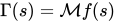
The Mellin transform of a complex-valued function
f
{\displaystyle f}
R
+
×
=
(
0
,
∞
)
{\displaystyle \mathbb {R} _{+}^{\times }=(0,\infty )}
M
f
{\displaystyle {\mathcal {M}}f}
s
{\displaystyle s}
M
{
f
}
(
s
)
=
φ
(
s
)
=
∫
0
∞
x
s
−
1
f
(
x
)
d
x
=
∫
R
+
×
f
(
x
)
x
s
d
x
x
.
{\displaystyle {\mathcal {M}}\left\{f\right\}(s)=\varphi (s)=\int _{0}^{\infty }x^{s-1}f(x)\,dx=\int _{\mathbb {R} _{+}^{\times }}f(x)x^{s}{\frac {dx}{x}}.}
d
x
/
x
{\displaystyle dx/x}
Haar measure on the multiplicative group
R
+
×
{\displaystyle \mathbb {R} _{+}^{\times }}
x
↦
x
s
{\displaystyle x\mapsto x^{s}}
multiplicative character . The inverse transform is given by
M
−
1
{
φ
}
(
x
)
=
f
(
x
)
=
1
2
π
i
∫
c
−
i
∞
c
+
i
∞
x
−
s
φ
(
s
)
d
s
.
{\displaystyle {\mathcal {M}}^{-1}\left\{\varphi \right\}(x)=f(x)={\frac {1}{2\pi i}}\int _{c-i\infty }^{c+i\infty }x^{-s}\varphi (s)\,ds.}
line integral over a vertical line in the complex plane , whose real part
c
{\displaystyle c}
Mellin inversion theorem .
The transform was introduced in 1859 by Bernhard Riemann . The transform is named after the Finnish mathematician Hjalmar Mellin , who developed the first rigorous treatment of the transform in 1897.[ 2]
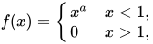
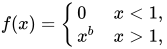
Polynomial functions [ edit ] Since
∫
0
∞
x
a
d
x
{\textstyle \int _{0}^{\infty }x^{a}dx}
a
∈
R
{\displaystyle a\in \mathbb {R} }
f
(
x
)
=
{
x
a
x
<
1
,
0
x
>
1
,
{\displaystyle f(x)={\begin{cases}x^{a}&x<1,\\0&x>1,\end{cases}}}
M
f
(
s
)
=
∫
0
1
x
s
−
1
x
a
d
x
=
∫
0
1
x
s
+
a
−
1
d
x
=
1
s
+
a
.
{\displaystyle {\mathcal {M}}f(s)=\int _{0}^{1}x^{s-1}x^{a}dx=\int _{0}^{1}x^{s+a-1}dx={\frac {1}{s+a}}.}
Hence
M
f
(
s
)
{\displaystyle {\mathcal {M}}f(s)}
s
=
−
a
{\displaystyle s=-a}
ℜ
(
s
)
>
−
a
{\displaystyle \Re (s)>-a}
f
(
x
)
=
{
0
x
<
1
,
x
b
x
>
1
,
{\displaystyle f(x)={\begin{cases}0&x<1,\\x^{b}&x>1,\end{cases}}}
M
f
(
s
)
=
∫
1
∞
x
s
−
1
x
b
d
x
=
∫
1
∞
x
s
+
b
−
1
d
x
=
−
1
s
+
b
.
{\displaystyle {\mathcal {M}}f(s)=\int _{1}^{\infty }x^{s-1}x^{b}dx=\int _{1}^{\infty }x^{s+b-1}dx=-{\frac {1}{s+b}}.}
M
f
(
s
)
{\displaystyle {\mathcal {M}}f(s)}
s
=
−
b
{\displaystyle s=-b}
ℜ
(
s
)
<
−
b
{\displaystyle \Re (s)<-b}
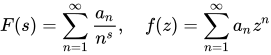
Power series and Dirichlet series [ edit ] Generally, assuming the necessary convergence, we can connect Dirichlet series and power series
F
(
s
)
=
∑
n
=
1
∞
a
n
n
s
,
f
(
z
)
=
∑
n
=
1
∞
a
n
z
n
{\displaystyle F(s)=\sum \limits _{n=1}^{\infty }{\frac {a_{n}}{n^{s}}},\quad f(z)=\sum \limits _{n=1}^{\infty }a_{n}z^{n}}
[ 5]
Γ
(
s
)
F
(
s
)
=
∫
0
∞
x
s
−
1
f
(
e
−
x
)
d
x
{\displaystyle \Gamma (s)F(s)=\int _{0}^{\infty }x^{s-1}f(e^{-x})dx}
For
α
,
β
∈
R
{\displaystyle \alpha ,\beta \in \mathbb {R} }
⟨
α
,
β
⟩
{\displaystyle \langle \alpha ,\beta \rangle }
s
∈
C
{\displaystyle s\in \mathbb {C} }
s
=
σ
+
i
t
{\displaystyle s=\sigma +it}
α
<
σ
<
β
{\displaystyle \alpha <\sigma <\beta }
fundamental strip of
M
f
(
s
)
{\displaystyle {\mathcal {M}}f(s)}
a
>
b
{\displaystyle a>b}
f
(
x
)
=
{
x
a
x
<
1
,
x
b
x
>
1
,
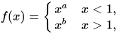
{\displaystyle f(x)={\begin{cases}x^{a}&x<1,\\x^{b}&x>1,\end{cases}}}
⟨
−
a
,
−
b
⟩
{\displaystyle \langle -a,-b\rangle }
x
→
0
+
{\displaystyle x\to 0^{+}}
x
→
+
∞
{\displaystyle x\to +\infty }
Big O notation , if
f
{\displaystyle f}
O
(
x
a
)
{\displaystyle O(x^{a})}
x
→
0
+
{\displaystyle x\to 0^{+}}
O
(
x
b
)
{\displaystyle O(x^{b})}
x
→
+
∞
{\displaystyle x\to +\infty }
M
f
(
s
)
{\displaystyle {\mathcal {M}}f(s)}
⟨
−
a
,
−
b
⟩
{\displaystyle \langle -a,-b\rangle }
An application of this can be seen in the gamma function,
Γ
(
s
)
{\displaystyle \Gamma (s)}
f
(
x
)
=
e
−
x
{\displaystyle f(x)=e^{-x}}
O
(
x
0
)
{\displaystyle O(x^{0})}
x
→
0
+
{\displaystyle x\to 0^{+}}
O
(
x
k
)
{\displaystyle O(x^{k})}
k
{\displaystyle k}
Γ
(
s
)
=
M
f
(
s
)
{\displaystyle \Gamma (s)={\mathcal {M}}f(s)}
⟨
0
,
+
∞
⟩
{\displaystyle \langle 0,+\infty \rangle }
Γ
(
s
)
{\displaystyle \Gamma (s)}
ℜ
(
s
)
>
0
{\displaystyle \Re (s)>0}
The properties in this table may be found in Bracewell (2000) and Erdélyi (1954) .
Properties of the Mellin transform
Function Mellin transform Fundamental strip Comments
f
(
x
)
{\displaystyle f(x)}
f
~
(
s
)
=
{
M
f
}
(
s
)
=
∫
0
∞
f
(
x
)
x
s
d
x
x
{\displaystyle {\tilde {f}}(s)=\{{\mathcal {M}}f\}(s)=\int _{0}^{\infty }f(x)x^{s}{\frac {dx}{x}}}
α
<
ℜ
s
<
β
{\displaystyle \alpha <\Re s<\beta }
Definition
x
ν
f
(
x
)
{\displaystyle x^{\nu }\,f(x)}
f
~
(
s
+
ν
)
{\displaystyle {\tilde {f}}(s+\nu )}
α
−
ℜ
ν
<
ℜ
s
<
β
−
ℜ
ν
{\displaystyle \alpha -\Re \nu <\Re s<\beta -\Re \nu }
f
(
x
ν
)
{\displaystyle f(x^{\nu })}
1
|
ν
|
f
~
(
s
ν
)
{\displaystyle {\frac {1}{|\nu |}}\,{\tilde {f}}\left({\frac {s}{\nu }}\right)}
α
<
ν
−
1
ℜ
s
<
β
{\displaystyle \alpha <\nu ^{-1}\,\Re s<\beta }
ν
∈
R
,
ν
≠
0
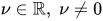
{\displaystyle \nu \in \mathbb {R} ,\;\nu \neq 0}
f
(
x
−
1
)
{\displaystyle f(x^{-1})}
f
~
(
−
s
)
{\displaystyle {\tilde {f}}(-s)}
−
β
<
ℜ
s
<
−
α
{\displaystyle -\beta <\Re s<-\alpha }
x
−
1
f
(
x
−
1
)
{\displaystyle x^{-1}\,f(x^{-1})}
f
~
(
1
−
s
)
{\displaystyle {\tilde {f}}(1-s)}
1
−
β
<
ℜ
s
<
1
−
α
{\displaystyle 1-\beta <\Re s<1-\alpha }
Involution
f
(
x
)
¯
{\displaystyle {\overline {f(x)}}}
f
~
(
s
¯
)
¯
{\displaystyle {\overline {{\tilde {f}}({\overline {s}})}}}
α
<
ℜ
s
<
β
{\displaystyle \alpha <\Re s<\beta }
Here
z
¯
{\displaystyle {\overline {z}}}
z
{\displaystyle z}
f
(
ν
x
)
{\displaystyle f(\nu x)}
ν
−
s
f
~
(
s
)
{\displaystyle \nu ^{-s}{\tilde {f}}(s)}
α
<
ℜ
s
<
β
{\displaystyle \alpha <\Re s<\beta }
ν
>
0
{\displaystyle \nu >0}
f
(
x
)
ln
x
{\displaystyle f(x)\,\ln x}
f
~
′
(
s
)
{\displaystyle {\tilde {f}}'(s)}
α
<
ℜ
s
<
β
{\displaystyle \alpha <\Re s<\beta }
f
′
(
x
)
{\displaystyle f'(x)}
−
(
s
−
1
)
f
~
(
s
−
1
)
{\displaystyle -(s-1)\,{\tilde {f}}(s-1)}
α
+
1
<
ℜ
s
<
β
+
1
{\displaystyle \alpha +1<\Re s<\beta +1}
The domain shift is conditional and requires evaluation against specific convergence behavior.
(
d
d
x
)
n
f
(
x
)
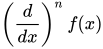
{\displaystyle \left({\frac {d}{dx}}\right)^{n}\,f(x)}
(
−
1
)
n
Γ
(
s
)
Γ
(
s
−
n
)
f
~
(
s
−
n
)
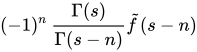
{\displaystyle (-1)^{n}\,{\frac {\Gamma (s)}{\Gamma (s-n)}}{\tilde {f}}(s-n)}
α
+
n
<
ℜ
s
<
β
+
n
{\displaystyle \alpha +n<\Re s<\beta +n}
x
f
′
(
x
)
{\displaystyle x\,f'(x)}
−
s
f
~
(
s
)
{\displaystyle -s\,{\tilde {f}}(s)}
α
<
ℜ
s
<
β
{\displaystyle \alpha <\Re s<\beta }
(
x
d
d
x
)
n
f
(
x
)
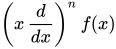
{\displaystyle \left(x\,{\frac {d}{dx}}\right)^{n}\,f(x)}
(
−
s
)
n
f
~
(
s
)
{\displaystyle (-s)^{n}{\tilde {f}}(s)}
α
<
ℜ
s
<
β
{\displaystyle \alpha <\Re s<\beta }
(
d
d
x
x
)
n
f
(
x
)
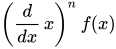
{\displaystyle \left({\frac {d}{dx}}\,x\right)^{n}\,f(x)}
(
1
−
s
)
n
f
~
(
s
)
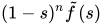
{\displaystyle (1-s)^{n}{\tilde {f}}(s)}
α
<
ℜ
s
<
β
{\displaystyle \alpha <\Re s<\beta }
∫
0
x
f
(
y
)
d
y
{\displaystyle \int _{0}^{x}f(y)\,dy}
−
s
−
1
f
~
(
s
+
1
)
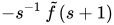
{\displaystyle -s^{-1}\,{\tilde {f}}(s+1)}
α
−
1
<
ℜ
s
<
min
(
β
−
1
,
0
)
{\displaystyle \alpha -1<\Re s<\min(\beta -1,0)}
Valid only if the integral exists.
∫
x
∞
f
(
y
)
d
y
{\displaystyle \int _{x}^{\infty }f(y)\,dy}
s
−
1
f
~
(
s
+
1
)
{\displaystyle s^{-1}\,{\tilde {f}}(s+1)}
max
(
α
−
1
,
0
)
<
ℜ
s
<
β
−
1
{\displaystyle \max(\alpha -1,0)<\Re s<\beta -1}
Valid only if the integral exists.
∫
0
∞
f
1
(
x
y
)
f
2
(
y
)
d
y
y
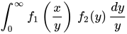
{\displaystyle \int _{0}^{\infty }f_{1}\left({\frac {x}{y}}\right)\,f_{2}(y)\,{\frac {dy}{y}}}
f
~
1
(
s
)
f
~
2
(
s
)
{\displaystyle {\tilde {f}}_{1}(s)\,{\tilde {f}}_{2}(s)}
max
(
α
1
,
α
2
)
<
ℜ
s
<
min
(
β
1
,
β
2
)
{\displaystyle \max(\alpha _{1},\alpha _{2})<\Re s<\min(\beta _{1},\beta _{2})}
Multiplicative convolution
x
μ
∫
0
∞
y
ν
f
1
(
x
y
)
f
2
(
y
)
d
y
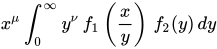
{\displaystyle x^{\mu }\int _{0}^{\infty }y^{\nu }\,f_{1}\left({\frac {x}{y}}\right)\,f_{2}(y)\,dy}
f
~
1
(
s
+
μ
)
f
~
2
(
s
+
μ
+
ν
+
1
)
{\displaystyle {\tilde {f}}_{1}(s+\mu )\,{\tilde {f}}_{2}(s+\mu +\nu +1)}
Multiplicative convolution (generalized)
x
μ
∫
0
∞
y
ν
f
1
(
x
y
)
f
2
(
y
)
d
y
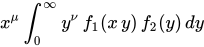
{\displaystyle x^{\mu }\int _{0}^{\infty }y^{\nu }\,f_{1}(x\,y)\,f_{2}(y)\,dy}
f
~
1
(
s
+
μ
)
f
~
2
(
1
−
s
−
μ
+
ν
)
{\displaystyle {\tilde {f}}_{1}(s+\mu )\,{\tilde {f}}_{2}(1-s-\mu +\nu )}
Multiplicative convolution (generalized)
f
1
(
x
)
f
2
(
x
)
{\displaystyle f_{1}(x)\,f_{2}(x)}
1
2
π
i
∫
c
−
i
∞
c
+
i
∞
f
~
1
(
r
)
f
~
2
(
s
−
r
)
d
r
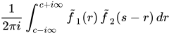
{\displaystyle {\frac {1}{2\pi i}}\int _{c-i\infty }^{c+i\infty }{\tilde {f}}_{1}(r)\,{\tilde {f}}_{2}(s-r)\,dr}
α
2
+
c
<
ℜ
s
<
β
2
+
c
α
1
<
c
<
β
1
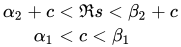
{\displaystyle {\begin{aligned}\alpha _{2}+c&<\Re s<\beta _{2}+c\\\alpha _{1}&<c<\beta _{1}\end{aligned}}}
Multiplication. Only valid if integral exists. See Parseval's theorem below for conditions which ensure the existence of the integral.
[ edit ] Let
f
1
(
x
)
{\displaystyle f_{1}(x)}
f
2
(
x
)
{\displaystyle f_{2}(x)}
f
~
1
,
2
(
s
)
=
M
{
f
1
,
2
}
(
s
)
{\displaystyle {\tilde {f}}_{1,2}(s)={\mathcal {M}}\{f_{1,2}\}(s)}
α
1
,
2
<
ℜ
s
<
β
1
,
2
{\displaystyle \alpha _{1,2}<\Re s<\beta _{1,2}}
c
∈
R
{\displaystyle c\in \mathbb {R} }
max
(
α
1
,
1
−
β
2
)
<
c
<
min
(
β
1
,
1
−
α
2
)
{\displaystyle \max(\alpha _{1},1-\beta _{2})<c<\min(\beta _{1},1-\alpha _{2})}
x
c
−
1
/
2
f
1
(
x
)
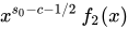
{\displaystyle x^{c-1/2}\,f_{1}(x)}
x
1
/
2
−
c
f
2
(
x
)
{\displaystyle x^{1/2-c}\,f_{2}(x)}
(
0
,
∞
)
{\displaystyle (0,\infty )}
Parseval's formula holds:
[ 7]
∫
0
∞
f
1
(
x
)
f
2
(
x
)
d
x
=
1
2
π
i
∫
c
−
i
∞
c
+
i
∞
f
1
~
(
s
)
f
2
~
(
1
−
s
)
d
s
{\displaystyle \int _{0}^{\infty }f_{1}(x)\,f_{2}(x)\,dx={\frac {1}{2\pi i}}\int _{c-i\infty }^{c+i\infty }{\tilde {f_{1}}}(s)\,{\tilde {f_{2}}}(1-s)\,ds}
ℜ
r
=
c
{\displaystyle \Re r=c}
We can replace
f
2
(
x
)
{\displaystyle f_{2}(x)}
f
2
(
x
)
x
s
0
−
1
{\displaystyle f_{2}(x)\,x^{s_{0}-1}}
f
1
(
x
)
{\displaystyle f_{1}(x)}
f
2
(
x
)
{\displaystyle f_{2}(x)}
f
~
1
,
2
(
s
)
=
M
{
f
1
,
2
}
(
s
)
{\displaystyle {\tilde {f}}_{1,2}(s)={\mathcal {M}}\{f_{1,2}\}(s)}
α
1
,
2
<
ℜ
s
<
β
1
,
2
{\displaystyle \alpha _{1,2}<\Re s<\beta _{1,2}}
c
∈
R
{\displaystyle c\in \mathbb {R} }
α
1
<
c
<
β
1
{\displaystyle \alpha _{1}<c<\beta _{1}}
s
0
∈
C
{\displaystyle s_{0}\in \mathbb {C} }
α
2
<
ℜ
s
0
−
c
<
β
2
{\displaystyle \alpha _{2}<\Re s_{0}-c<\beta _{2}}
x
c
−
1
/
2
f
1
(
x
)
{\displaystyle x^{c-1/2}\,f_{1}(x)}
x
s
0
−
c
−
1
/
2
f
2
(
x
)
{\displaystyle x^{s_{0}-c-1/2}\,f_{2}(x)}
(
0
,
∞
)
{\displaystyle (0,\infty )}
[ 7]
∫
0
∞
f
1
(
x
)
f
2
(
x
)
x
s
0
−
1
d
x
=
1
2
π
i
∫
c
−
i
∞
c
+
i
∞
f
1
~
(
s
)
f
2
~
(
s
0
−
s
)
d
s
{\displaystyle \int _{0}^{\infty }f_{1}(x)\,f_{2}(x)\,x^{s_{0}-1}\,dx={\frac {1}{2\pi i}}\int _{c-i\infty }^{c+i\infty }{\tilde {f_{1}}}(s)\,{\tilde {f_{2}}}(s_{0}-s)\,ds}
f
2
(
x
)
{\displaystyle f_{2}(x)}
f
1
(
x
)
¯
{\displaystyle {\overline {f_{1}(x)}}}
f
(
x
)
{\displaystyle f(x)}
f
~
(
s
)
=
M
{
f
}
(
s
)
{\displaystyle {\tilde {f}}(s)={\mathcal {M}}\{f\}(s)}
α
<
ℜ
s
<
β
{\displaystyle \alpha <\Re s<\beta }
c
∈
R
{\displaystyle c\in \mathbb {R} }
α
<
c
<
β
{\displaystyle \alpha <c<\beta }
x
c
−
1
/
2
f
(
x
)
{\displaystyle x^{c-1/2}\,f(x)}
(
0
,
∞
)
{\displaystyle (0,\infty )}
Plancherel's theorem holds:[ 8]
∫
0
∞
|
f
(
x
)
|
2
x
2
c
−
1
d
x
=
1
2
π
∫
−
∞
∞
|
f
~
(
c
+
i
t
)
|
2
d
t
{\displaystyle \int _{0}^{\infty }|f(x)|^{2}\,x^{2c-1}dx={\frac {1}{2\pi }}\int _{-\infty }^{\infty }|{\tilde {f}}(c+it)|^{2}\,dt}
As an isometry on L 2 spaces [ edit ] In the study of Hilbert spaces , the Mellin transform is often posed in a slightly different way. For functions in
L
2
(
0
,
∞
)
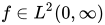
{\displaystyle L^{2}(0,\infty )}
L p
1
2
+
i
R
{\displaystyle {\tfrac {1}{2}}+i\mathbb {R} }
linear operator
M
~
{\displaystyle {\tilde {\mathcal {M}}}}
M
~
:
L
2
(
0
,
∞
)
→
L
2
(
−
∞
,
∞
)
,
{\displaystyle {\tilde {\mathcal {M}}}\colon L^{2}(0,\infty )\to L^{2}(-\infty ,\infty ),}
{
M
~
f
}
(
s
)
:=
1
2
π
∫
0
∞
x
−
1
2
+
i
s
f
(
x
)
d
x
.
{\displaystyle \{{\tilde {\mathcal {M}}}f\}(s):={\frac {1}{\sqrt {2\pi }}}\int _{0}^{\infty }x^{-{\frac {1}{2}}+is}f(x)\,dx.}
{
M
~
f
}
(
s
)
:=
1
2
π
{
M
f
}
(
1
2
+
i
s
)
.
{\displaystyle \{{\tilde {\mathcal {M}}}f\}(s):={\tfrac {1}{\sqrt {2\pi }}}\{{\mathcal {M}}f\}({\tfrac {1}{2}}+is).}
M
{\displaystyle {\mathcal {M}}}
M
~
{\displaystyle {\tilde {\mathcal {M}}}}
Mellin inversion theorem then shows that
M
~
{\displaystyle {\tilde {\mathcal {M}}}}
M
~
−
1
:
L
2
(
−
∞
,
∞
)
→
L
2
(
0
,
∞
)
,
{\displaystyle {\tilde {\mathcal {M}}}^{-1}\colon L^{2}(-\infty ,\infty )\to L^{2}(0,\infty ),}
{
M
~
−
1
φ
}
(
x
)
=
1
2
π
∫
−
∞
∞
x
−
1
2
−
i
s
φ
(
s
)
d
s
.
{\displaystyle \{{\tilde {\mathcal {M}}}^{-1}\varphi \}(x)={\frac {1}{\sqrt {2\pi }}}\int _{-\infty }^{\infty }x^{-{\frac {1}{2}}-is}\varphi (s)\,ds.}
isometry , that is to say
‖
M
~
f
‖
L
2
(
−
∞
,
∞
)
=
‖
f
‖
L
2
(
0
,
∞
)
{\displaystyle \|{\tilde {\mathcal {M}}}f\|_{L^{2}(-\infty ,\infty )}=\|f\|_{L^{2}(0,\infty )}}
f
∈
L
2
(
0
,
∞
)
{\displaystyle f\in L^{2}(0,\infty )}
1
/
2
π
{\displaystyle 1/{\sqrt {2\pi }}}
In probability theory [ edit ] In probability theory , the Mellin transform is an essential tool in studying the distributions of products of random variables.[ 9]
X
{\displaystyle X}
random variable , and
X
+
=
max
{
X
,
0
}
{\displaystyle X^{+}=\max\{X,0\}}
X
−
=
max
{
−
X
,
0
}
{\displaystyle X^{-}=\max\{-X,0\}}
Mellin transform of
X
{\displaystyle X}
[ 10]
M
X
(
s
)
=
∫
0
∞
x
s
d
F
X
+
(
x
)
+
γ
∫
0
∞
x
s
d
F
X
−
(
x
)
,
{\displaystyle {\mathcal {M}}_{X}(s)=\int _{0}^{\infty }x^{s}dF_{X^{+}}(x)+\gamma \int _{0}^{\infty }x^{s}dF_{X^{-}}(x),}
γ
{\displaystyle \gamma }
γ
2
=
1
{\displaystyle \gamma ^{2}=1}
s
{\displaystyle s}
D
=
{
s
:
a
≤
ℜ
(
s
)
≤
b
}
{\displaystyle D=\{s:a\leq \Re (s)\leq b\}}
a
≤
0
≤
b
{\displaystyle a\leq 0\leq b}
[ 10]
The Mellin transform
M
X
(
i
t
)
{\displaystyle {\mathcal {M}}_{X}(it)}
X
{\displaystyle X}
F
X
{\displaystyle F_{X}}
[ 10]
X
{\displaystyle X}
Y
{\displaystyle Y}
X
{\displaystyle X}
Y
{\displaystyle Y}
[ 11]
M
X
Y
(
s
)
=
M
X
(
s
)
M
Y
(
s
)
{\displaystyle {\mathcal {M}}_{XY}(s)={\mathcal {M}}_{X}(s){\mathcal {M}}_{Y}(s)}
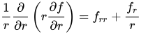
Problems with Laplacian in cylindrical coordinate system [ edit ] In the Laplacian in cylindrical coordinates in a generic dimension (orthogonal coordinates with one angle and one radius, and the remaining lengths) there is always a term:
1
r
∂
∂
r
(
r
∂
f
∂
r
)
=
f
r
r
+
f
r
r
{\displaystyle {\frac {1}{r}}{\frac {\partial }{\partial r}}\left(r{\frac {\partial f}{\partial r}}\right)=f_{rr}+{\frac {f_{r}}{r}}}
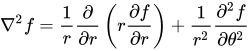
For example, in 2-D polar coordinates the Laplacian is:
∇
2
f
=
1
r
∂
∂
r
(
r
∂
f
∂
r
)
+
1
r
2
∂
2
f
∂
θ
2
{\displaystyle \nabla ^{2}f={\frac {1}{r}}{\frac {\partial }{\partial r}}\left(r{\frac {\partial f}{\partial r}}\right)+{\frac {1}{r^{2}}}{\frac {\partial ^{2}f}{\partial \theta ^{2}}}}
∇
2
f
=
1
r
∂
∂
r
(
r
∂
f
∂
r
)
+
1
r
2
∂
2
f
∂
φ
2
+
∂
2
f
∂
z
2
.
{\displaystyle \nabla ^{2}f={\frac {1}{r}}{\frac {\partial }{\partial r}}\left(r{\frac {\partial f}{\partial r}}\right)+{\frac {1}{r^{2}}}{\frac {\partial ^{2}f}{\partial \varphi ^{2}}}+{\frac {\partial ^{2}f}{\partial z^{2}}}.}
This term can be treated with the Mellin transform,[ 12]
M
(
r
2
f
r
r
+
r
f
r
,
r
→
s
)
=
s
2
M
(
f
,
r
→
s
)
=
s
2
F
{\displaystyle {\mathcal {M}}\left(r^{2}f_{rr}+rf_{r},r\to s\right)=s^{2}{\mathcal {M}}\left(f,r\to s\right)=s^{2}F}
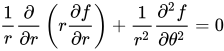
For example, the 2-D Laplace equation in polar coordinates is the PDE in two variables:
r
2
f
r
r
+
r
f
r
+
f
θ
θ
=
0
{\displaystyle r^{2}f_{rr}+rf_{r}+f_{\theta \theta }=0}
1
r
∂
∂
r
(
r
∂
f
∂
r
)
+
1
r
2
∂
2
f
∂
θ
2
=
0
{\displaystyle {\frac {1}{r}}{\frac {\partial }{\partial r}}\left(r{\frac {\partial f}{\partial r}}\right)+{\frac {1}{r^{2}}}{\frac {\partial ^{2}f}{\partial \theta ^{2}}}=0}
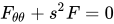
harmonic oscillator :
F
θ
θ
+
s
2
F
=
0
{\displaystyle F_{\theta \theta }+s^{2}F=0}
F
(
s
,
θ
)
=
C
1
(
s
)
cos
(
s
θ
)
+
C
2
(
s
)
sin
(
s
θ
)
{\displaystyle F(s,\theta )=C_{1}(s)\cos(s\theta )+C_{2}(s)\sin(s\theta )}
Now let's impose for example some simple wedge boundary conditions to the original Laplace equation:
f
(
r
,
−
θ
0
)
=
a
(
r
)
,
f
(
r
,
θ
0
)
=
b
(
r
)
{\displaystyle f(r,-\theta _{0})=a(r),\quad f(r,\theta _{0})=b(r)}
F
(
s
,
−
θ
0
)
=
A
(
s
)
,
F
(
s
,
θ
0
)
=
B
(
s
)
{\displaystyle F(s,-\theta _{0})=A(s),\quad F(s,\theta _{0})=B(s)}
These conditions imposed to the solution particularize it to:
F
(
s
,
θ
)
=
A
(
s
)
sin
(
s
(
θ
0
−
θ
)
)
sin
(
2
θ
0
s
)
+
B
(
s
)
sin
(
s
(
θ
0
+
θ
)
)
sin
(
2
θ
0
s
)
{\displaystyle F(s,\theta )=A(s){\frac {\sin(s(\theta _{0}-\theta ))}{\sin(2\theta _{0}s)}}+B(s){\frac {\sin(s(\theta _{0}+\theta ))}{\sin(2\theta _{0}s)}}}
Now by the convolution theorem for Mellin transform, the solution in the Mellin domain can be inverted:
f
(
r
,
θ
)
=
r
m
cos
(
m
θ
)
2
θ
0
∫
0
∞
(
a
(
x
)
x
2
m
+
2
r
m
x
m
sin
(
m
θ
)
+
r
2
m
+
b
(
x
)
x
2
m
−
2
r
m
x
m
sin
(
m
θ
)
+
r
2
m
)
x
m
−
1
d
x
{\displaystyle f(r,\theta )={\frac {r^{m}\cos(m\theta )}{2\theta _{0}}}\int _{0}^{\infty }\left({\frac {a(x)}{x^{2m}+2r^{m}x^{m}\sin(m\theta )+r^{2m}}}+{\frac {b(x)}{x^{2m}-2r^{m}x^{m}\sin(m\theta )+r^{2m}}}\right)x^{m-1}\,dx}
M
−
1
(
sin
(
s
φ
)
sin
(
2
θ
0
s
)
;
s
→
r
)
=
1
2
θ
0
r
m
sin
(
m
φ
)
1
+
2
r
m
cos
(
m
φ
)
+
r
2
m
{\displaystyle {\mathcal {M}}^{-1}\left({\frac {\sin(s\varphi )}{\sin(2\theta _{0}s)}};s\to r\right)={\frac {1}{2\theta _{0}}}{\frac {r^{m}\sin(m\varphi )}{1+2r^{m}\cos(m\varphi )+r^{2m}}}}
m
=
π
2
θ
0
{\displaystyle m={\frac {\pi }{2\theta _{0}}}}
Below is a list of interesting examples for the Mellin transform:
Selected Mellin transforms
Function
f
(
x
)
{\displaystyle f(x)}
Mellin transform
f
~
(
s
)
=
M
{
f
}
(
s
)
{\displaystyle {\tilde {f}}(s)={\mathcal {M}}\{f\}(s)}
Region of convergence
Comment
e
−
x
{\displaystyle e^{-x}}
Γ
(
s
)
{\displaystyle \Gamma (s)}
0
<
ℜ
s
<
∞
{\displaystyle 0<\Re s<\infty }
e
−
x
−
1
{\displaystyle e^{-x}-1}
Γ
(
s
)
{\displaystyle \Gamma (s)}
−
1
<
ℜ
s
<
0
{\displaystyle -1<\Re s<0}
e
−
x
−
1
+
x
{\displaystyle e^{-x}-1+x}
Γ
(
s
)
{\displaystyle \Gamma (s)}
−
2
<
ℜ
s
<
−
1
{\displaystyle -2<\Re s<-1}
Generally
Γ
(
s
)
{\displaystyle \Gamma (s)}
[ 18]
e
−
x
−
∑
n
=
0
N
−
1
(
−
1
)
n
n
!
x
n
{\displaystyle \textstyle e^{-x}-\sum _{n=0}^{N-1}{\frac {(-1)^{n}}{n!}}x^{n}}
for
−
N
<
ℜ
s
<
−
N
+
1
{\displaystyle -N<\Re s<-N+1}
e
−
x
2
{\displaystyle e^{-x^{2}}}
1
2
Γ
(
1
2
s
)
{\displaystyle {\tfrac {1}{2}}\Gamma ({\tfrac {1}{2}}s)}
0
<
ℜ
s
<
∞
{\displaystyle 0<\Re s<\infty }
e
r
f
c
(
x
)
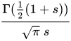
{\displaystyle \mathrm {erfc} (x)}
Γ
(
1
2
(
1
+
s
)
)
π
s
{\displaystyle {\frac {\Gamma ({\tfrac {1}{2}}(1+s))}{{\sqrt {\pi }}\;s}}}
0
<
ℜ
s
<
∞
{\displaystyle 0<\Re s<\infty }
e
−
(
ln
x
)
2
{\displaystyle e^{-(\ln x)^{2}}}
π
e
1
4
s
2
{\displaystyle {\sqrt {\pi }}\,e^{{\tfrac {1}{4}}s^{2}}}
−
∞
<
ℜ
s
<
∞
{\displaystyle -\infty <\Re s<\infty }
δ
(
x
−
a
)
{\displaystyle \delta (x-a)}
a
s
−
1
{\displaystyle a^{s-1}}
−
∞
<
ℜ
s
<
∞
{\displaystyle -\infty <\Re s<\infty }
a
>
0
,
δ
(
x
)
{\displaystyle a>0,\;\delta (x)}
Dirac delta function
u
(
1
−
x
)
=
{
1
if
0
<
x
<
1
0
if
1
<
x
<
∞
{\displaystyle u(1-x)=\left\{{\begin{aligned}&1&&\;{\text{if}}\;0<x<1&\\&0&&\;{\text{if}}\;1<x<\infty &\end{aligned}}\right.}
1
s
{\displaystyle {\frac {1}{s}}}
0
<
ℜ
s
<
∞
{\displaystyle 0<\Re s<\infty }
u
(
x
)
{\displaystyle u(x)}
Heaviside step function
−
u
(
x
−
1
)
=
{
0
if
0
<
x
<
1
−
1
if
1
<
x
<
∞
{\displaystyle -u(x-1)=\left\{{\begin{aligned}&0&&\;{\text{if}}\;0<x<1&\\&-1&&\;{\text{if}}\;1<x<\infty &\end{aligned}}\right.}
1
s
{\displaystyle {\frac {1}{s}}}
−
∞
<
ℜ
s
<
0
{\displaystyle -\infty <\Re s<0}
u
(
1
−
x
)
x
a
=
{
x
a
if
0
<
x
<
1
0
if
1
<
x
<
∞
{\displaystyle u(1-x)\,x^{a}=\left\{{\begin{aligned}&x^{a}&&\;{\text{if}}\;0<x<1&\\&0&&\;{\text{if}}\;1<x<\infty &\end{aligned}}\right.}
1
s
+
a
{\displaystyle {\frac {1}{s+a}}}
−
ℜ
a
<
ℜ
s
<
∞
{\displaystyle -\Re a<\Re s<\infty }
−
u
(
x
−
1
)
x
a
=
{
0
if
0
<
x
<
1
−
x
a
if
1
<
x
<
∞
{\displaystyle -u(x-1)\,x^{a}=\left\{{\begin{aligned}&0&&\;{\text{if}}\;0<x<1&\\&-x^{a}&&\;{\text{if}}\;1<x<\infty &\end{aligned}}\right.}
1
s
+
a
{\displaystyle {\frac {1}{s+a}}}
−
∞
<
ℜ
s
<
−
ℜ
a
{\displaystyle -\infty <\Re s<-\Re a}
u
(
1
−
x
)
x
a
ln
x
=
{
x
a
ln
x
if
0
<
x
<
1
0
if
1
<
x
<
∞
{\displaystyle u(1-x)\,x^{a}\ln x=\left\{{\begin{aligned}&x^{a}\ln x&&\;{\text{if}}\;0<x<1&\\&0&&\;{\text{if}}\;1<x<\infty &\end{aligned}}\right.}
1
(
s
+
a
)
2
{\displaystyle {\frac {1}{(s+a)^{2}}}}
−
ℜ
a
<
ℜ
s
<
∞
{\displaystyle -\Re a<\Re s<\infty }
−
u
(
x
−
1
)
x
a
ln
x
=
{
0
if
0
<
x
<
1
−
x
a
ln
x
if
1
<
x
<
∞
{\displaystyle -u(x-1)\,x^{a}\ln x=\left\{{\begin{aligned}&0&&\;{\text{if}}\;0<x<1&\\&-x^{a}\ln x&&\;{\text{if}}\;1<x<\infty &\end{aligned}}\right.}
1
(
s
+
a
)
2
{\displaystyle {\frac {1}{(s+a)^{2}}}}
−
∞
<
ℜ
s
<
−
ℜ
a
{\displaystyle -\infty <\Re s<-\Re a}
1
1
+
x
{\displaystyle {\frac {1}{1+x}}}
π
sin
(
π
s
)
{\displaystyle {\frac {\pi }{\sin(\pi s)}}}
0
<
ℜ
s
<
1
{\displaystyle 0<\Re s<1}
1
1
−
x
{\displaystyle {\frac {1}{1-x}}}
π
tan
(
π
s
)
{\displaystyle {\frac {\pi }{\tan(\pi s)}}}
0
<
ℜ
s
<
1
{\displaystyle 0<\Re s<1}
The integral uses the Cauchy principal value .
1
1
+
x
2
{\displaystyle {\frac {1}{1+x^{2}}}}
π
2
sin
(
1
2
π
s
)
{\displaystyle {\frac {\pi }{2\sin({\tfrac {1}{2}}\pi s)}}}
0
<
ℜ
s
<
2
{\displaystyle 0<\Re s<2}
1
(
1
+
x
)
a
{\displaystyle {\frac {1}{(1+x)^{a}}}}
Γ
(
s
)
Γ
(
a
−
s
)
Γ
(
a
)
{\displaystyle {\frac {\Gamma (s)\,\Gamma (a-s)}{\Gamma (a)}}}
0
<
ℜ
s
<
ℜ
a
{\displaystyle 0<\Re s<\Re a}
Binomial series
u
(
1
−
x
)
(
1
−
x
)
a
−
1
{\displaystyle u(1-x)\;(1-x)^{a-1}}
Γ
(
s
)
Γ
(
a
)
Γ
(
s
+
a
)
{\displaystyle {\frac {\Gamma (s)\,\Gamma (a)}{\Gamma (s+a)}}}
0
<
ℜ
s
<
∞
{\displaystyle 0<\Re s<\infty }
ℜ
a
>
0
{\displaystyle \Re a>0}
u
(
x
−
1
)
(
1
−
x
)
−
a
{\displaystyle u(x-1)\;(1-x)^{-a}}
Γ
(
a
−
s
)
Γ
(
1
−
a
)
Γ
(
1
−
s
)
{\displaystyle {\frac {\Gamma (a-s)\,\Gamma (1-a)}{\Gamma (1-s)}}}
−
∞
<
ℜ
s
<
ℜ
a
{\displaystyle -\infty <\Re s<\Re a}
ℜ
a
<
1
{\displaystyle \Re a<1}
ln
(
1
+
x
)
{\displaystyle \ln(1+x)}
π
s
sin
(
π
s
)
{\displaystyle {\frac {\pi }{s\,\sin(\pi s)}}}
−
1
<
ℜ
s
<
0
{\displaystyle -1<\Re s<0}
ln
|
1
−
x
|
{\displaystyle \ln \vert 1-x\vert }
π
s
cot
(
π
s
)
{\displaystyle {\frac {\pi }{s}}\,\cot(\pi s)}
−
1
<
ℜ
s
<
0
{\displaystyle -1<\Re s<0}
acot
x
=
π
2
−
atan
x
{\displaystyle \operatorname {acot} x={\frac {\pi }{2}}-\operatorname {atan} x}
π
2
s
cos
(
π
s
/
2
)
{\displaystyle {\frac {\pi }{2s\,\cos(\pi s/2)}}}
0
<
ℜ
s
<
1
{\displaystyle 0<\Re s<1}
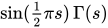
sin
(
x
)
{\displaystyle \sin(x)}
sin
(
1
2
π
s
)
Γ
(
s
)
{\displaystyle \sin({\tfrac {1}{2}}\pi s)\,\Gamma (s)}
−
1
<
ℜ
s
<
1
{\displaystyle -1<\Re s<1}
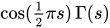
cos
(
x
)
{\displaystyle \cos(x)}
cos
(
1
2
π
s
)
Γ
(
s
)
{\displaystyle \cos({\tfrac {1}{2}}\pi s)\,\Gamma (s)}
0
<
ℜ
s
<
1
{\displaystyle 0<\Re s<1}
e
i
x
{\displaystyle e^{ix}}
e
i
π
s
/
2
Γ
(
s
)
{\displaystyle e^{i\pi s/2}\,\Gamma (s)}
0
<
ℜ
s
<
1
{\displaystyle 0<\Re s<1}
J
0
(
x
)
{\displaystyle J_{0}(x)}
2
s
−
1
π
sin
(
π
s
/
2
)
[
Γ
(
s
/
2
)
]
2
{\displaystyle {\frac {2^{s-1}}{\pi }}\,\sin(\pi s/2)\,\left[\Gamma (s/2)\right]^{2}}
0
<
ℜ
s
<
3
2
{\displaystyle 0<\Re s<{\tfrac {3}{2}}}
J
0
(
x
)
{\displaystyle J_{0}(x)}
Bessel function of the first kind.
Y
0
(
x
)
{\displaystyle Y_{0}(x)}
−
2
s
−
1
π
cos
(
π
s
/
2
)
[
Γ
(
s
/
2
)
]
2
{\displaystyle -{\frac {2^{s-1}}{\pi }}\,\cos(\pi s/2)\,\left[\Gamma (s/2)\right]^{2}}
0
<
ℜ
s
<
3
2
{\displaystyle 0<\Re s<{\tfrac {3}{2}}}
Y
0
(
x
)
{\displaystyle Y_{0}(x)}
Bessel function of the second kind
K
0
(
x
)
{\displaystyle K_{0}(x)}
2
s
−
2
[
Γ
(
s
/
2
)
]
2
{\displaystyle 2^{s-2}\,\left[\Gamma (s/2)\right]^{2}}
0
<
ℜ
s
<
∞
{\displaystyle 0<\Re s<\infty }
K
0
(
x
)
{\displaystyle K_{0}(x)}
Bessel function of the second kind
↑ Mellin, Hj. "Zur Theorie zweier allgemeinen Klassen bestimmter Integrale" . Acta Societatis Scientiarum Fennicae (in German). XXII (2).↑ Whittaker, E. T. ; Watson, G. N. (1996). A Course of Modern Analysis ↑ Hardy, G. H. ; Littlewood, J. E. (1916). "Contributions to the Theory of the Riemann Zeta-Function and the Theory of the Distribution of Primes" . Acta Mathematica 41 (1): 119– 196. doi :10.1007/BF02422942 See notes therein for further references to Cahen's and Mellin's work, including Cahen's thesis. )↑ Wintner, Aurel (1947). "On Riemann's Reduction of Dirichlet Series to Power Series" . American Journal of Mathematics 69 (4): 769– 789. doi :10.2307/2371798 JSTOR 2371798 .1 2 Titchmarsh (1948 , p. 95) .↑ Titchmarsh (1948 , p. 94) .↑ Galambos & Simonelli (2004 , p. 15) 1 2 3 Galambos & Simonelli (2004 , p. 16) ↑ Galambos & Simonelli (2004 , p. 23) ↑ Bhimsen, Shivamoggi, Chapter 6: The Mellin Transform, par. 4.3: Distribution of a Potential in a Wedge, pp. 267–268 ↑ Philippe Flajolet and Robert Sedgewick. The Average Case Analysis of Algorithms: Mellin Transform Asymptotics. Research Report 2956. 93 pages. Institut National de Recherche en Informatique et en Automatique (INRIA), 1996. ↑ A. Liam Fitzpatrick, Jared Kaplan, Joao Penedones, Suvrat Raju, Balt C. van Rees. "A Natural Language for AdS/CFT Correlators" . ↑ A. Liam Fitzpatrick, Jared Kaplan. "Unitarity and the Holographic S-Matrix" ↑ A. Liam Fitzpatrick. "AdS/CFT and the Holographic S-Matrix" , video lecture. ↑ Bertrand, Jacqueline; Bertrand, Pierre; Ovarlez, Jean-Philippe (1995). The Mellin Transform: The Transforms and Applications Handbook . Taylor & Francis. ISBN 978-1420066524
Bracewell, Ronald N. (2000). The Fourier Transform and Its Applications (3rd ed.). Debnath, Lokenath; Bhatta, Dambaru (19 April 2016). Integral Transforms and Their Applications ISBN 978-1-4200-1091-6 Epstein, Benjamin. "Some Applications of the Mellin Transform in Statistics" . Carnegie Mellon Institute of Technology. Erdélyi, Arthur (1954). Tables of Integral Transforms . Vol. 1. McGraw-Hill. Flajolet, P.; Gourdon, X.; Dumas, P. (1995). "Mellin transforms and asymptotics: Harmonic sums" (PDF) . Theoretical Computer Science . 144 (1– 2): 3– 58. doi :10.1016/0304-3975(95)00002-e . Galambos, Janos; Simonelli, Italo (2004). Products of random variables: applications to problems of physics and to arithmetical functions ISBN 0-8247-5402-6 Paris, R. B.; Kaminski, D. (2001). Asymptotics and Mellin-Barnes Integrals ISBN 9780521790017 Polyanin, A. D.; Manzhirov, A. V. (1998). Handbook of Integral Equations . Boca Raton, Florida: CRC Press. ISBN 0-8493-2876-4 Titchmarsh, E. C. (1948). Introduction to the Theory of Fourier Integrals (2nd ed.). Polyanin, Andrei D. "Tables of Integral Transforms" . EqWorld: The World of Mathematical Equations . "Mellin transform" , Encyclopedia of Mathematics Weisstein, Eric W. "Mellin Transform" . MathWorld
Philippe Flajolet, Xavier Gourdon, Philippe Dumas, Mellin Transforms and Asymptotics: Harmonic sums
Antonio Gonzáles, Marko Riedel Celebrando un clásico , newsgroup es.ciencia.matematicas
Juan Sacerdoti, Funciones Eulerianas
Mellin Transform Methods , Digital Library of Mathematical Functions , 2011-08-29, National Institute of Standards and Technology Antonio De Sena and Davide Rocchesso, A Fast Mellin Transform with Applications in DAFX

















































































































































![{\displaystyle {\frac {2^{s-1}}{\pi }}\,\sin(\pi s/2)\,\left[\Gamma (s/2)\right]^{2}}](https://wikimedia.org/api/rest_v1/media/math/render/svg/4d0e885f459fbb32e29613b2472f4afc5e82aab9)


![{\displaystyle -{\frac {2^{s-1}}{\pi }}\,\cos(\pi s/2)\,\left[\Gamma (s/2)\right]^{2}}](https://wikimedia.org/api/rest_v1/media/math/render/svg/ab65fcf0eb4e99b5e78eb11650c4fd781f8df2d3)

![{\displaystyle 2^{s-2}\,\left[\Gamma (s/2)\right]^{2}}](https://wikimedia.org/api/rest_v1/media/math/render/svg/5eb045a02da01962eced207026a375234296ba0a)