// Workers AI · dad joke modeWhat did marginal product say? "I'm on the edge.

Average physical product (APP), marginal physical product (MPP)

In economics and in particular neoclassical economics, the marginal product or marginal physical productivity of an input (factor of production) is the change in output resulting from employing one more unit of a particular input (for instance, the change in output when a firm's labor is increased from five to six units), assuming that the quantities of other inputs are kept constant.

The marginal product of a given input can be expressed as:

$MP={\frac {\Delta Y}{\Delta X}}$

where $\Delta X$ is the change in the firm's use of the input (conventionally a one-unit change) and $\Delta Y$ is the change in the quantity of output produced (resulting from the change in the input). Note that the quantity $Y$ of the "product" is typically defined ignoring external costs and benefits.

If the output and the input are infinitely divisible, so the marginal "units" are infinitesimal, the marginal product is the mathematical derivative of the production function with respect to that input. Suppose a firm's output Y is given by the production function:

$Y=F(K,L)$

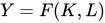
where K and L are inputs to production (say, capital and labor, respectively). Then the marginal product of capital (MPK) and marginal product of labor (MPL) are given by:

$MPK={\frac {\partial F}{\partial K}}$

$MPL={\frac {\partial F}{\partial L}}$

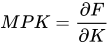
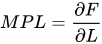
In the law of diminishing marginal returns, the marginal product initially increases when more of an input (say labor) is employed, keeping the other input (say capital) constant. Here, labor is the variable input and capital is the fixed input (in a hypothetical two-inputs model). As more and more of variable input (labor) is employed, marginal product starts to fall. Finally, after a certain point, the marginal product becomes negative, implying that the additional unit of labor has decreased the output, rather than increasing it. The reason behind this is the diminishing marginal productivity of labor.

The marginal product of labor is the slope of the total product curve, which is the production function plotted against labor usage for a fixed level of usage of the capital input.

In the neoclassical theory of competitive markets, the marginal product of labor equals the real wage. In aggregate models of perfect competition, in which a single good is produced and that good is used both in consumption and as a capital good, the marginal product of capital equals its rate of return. As was shown in the Cambridge capital controversy, this proposition about the marginal product of capital cannot generally be sustained in multi-commodity models in which capital and consumption goods are distinguished.

Relationship of marginal product (MPP) with the total product (TPP)

The relationship can be explained in three phases- (1) Initially, as the quantity of variable input is increased, TPP rises at an increasing rate. In this phase, MPP also rises. (2) As more and more quantities of the variable inputs are employed, TPP increases at a diminishing rate. In this phase, MPP starts to fall. (3) When the TPP reaches its maximum, MPP is zero. Beyond this point, TPP starts to fall and MPP becomes negative.

The concept of the relationship between marginal product and the law of diminishing marginal returns is better explained by the three stages of production, which characterised the behaviour of total physical product (TPP) and marginal physical product (MPP) as a variable input changes, assuming at least one input remains constant .

The range of production in which MPP is growing is encompassed in stage I. The variable input becomes more specialised the more units of the variable input are added to the fixed input, and the fixed input is used more frequently. An increasing rate of output occurs when a unit increase in the variable input adds more to production with each successive increase. A business in Stage I would never stop using additional variable input because it hasn't yet fully utilised its fixed input. This is why Stage II is no longer viewed as a rational termination point of a profit-maximising firm . Stage II is the period of maximum MPP, and when it begins to decay, stage II ends at zero MPP. The total output at the stage goes on increasing, though at a slowing pace, which is an indicator of originating diminishing marginal returns as the fixed input is increasingly crowded in comparison to the change in the variable input . The economically viable span of production is only stage II for a firm ready to maximise profits. In this range, the extra units of the variable input continue to increase total output, and the firm can evaluate the marginal product of an extra unit of input and compare this with the cost of that extra unit of input to make a decision on the level of employment that maximises profits. . Stage III starts when MPP is less than zero. The variable input is so plentiful in comparison with the fixed input that extra units are actively decreasing the total output. This is a situation called 'input crowding'. In Stage II, no profit-maximising firm would knowingly act in Stage III because, by employing an extra unit of input and yielding less output, a firm maximising its profit would have the characteristics of raising both costs and revenue at the same time . Using the example of a fixed piece of land where people are also workers, we can discuss this. Few workers would be employed, and a single extra worker would increase the output significantly, putting the firm in Stage I. The more workers are recruited, the more the output increases, but the contributions by each worker are lower than those of the others due to Stage II. When the hiring is not stopped, when the land becomes completely congested, the workers start to disrupt each other, and the overall production is reduced, which is a sign of Stage III.

Stage	TPP	MPP
Stage I	Rising at an increasing rate	Rising
Stage II	Rising at a decreasing rate	Positive but falling
Stage III	Falling	Negative

See also

• Marginal product of labor
• Marginal product of capital
• Marginal revenue productivity theory of wages
• Marginal cost
• Production theory
• Average product
• Cost of production
• Shadow price

Further reading

• Beck, Bernhard (2008). Volkswirtschaft verstehen. vdf, Hochsch.-Verlag an der ETH. ISBN 978-3-7281-3207-9.
• Rothbard, Murray N. (1995). Classical Economics: An Austrian Perspective on the History of Economic Thought, Volume II (PDF). Auburn, Alabama: Ludwig von Mises Institute. ISBN 0-945466-48-X.