Hermite interpolation

In numerical analysis, Hermite interpolation, named after Charles Hermite, is a method of polynomial interpolation, which generalizes Lagrange interpolation. Lagrange interpolation allows computing a polynomial of degree less than n that takes the same value at n given points as a given function. Instead, Hermite interpolation computes a polynomial of degree fewer than n such that the polynomial and its first few derivatives have the same values at m (fewer than n) given points as the given function and its first few derivatives at those points. The number of pieces of information, function values and derivative values, must add up to $n$.

Hermite's method of interpolation is closely related to the Newton's interpolation method, in that both can be derived from the calculation of divided differences. However, there are other methods for computing a Hermite interpolating polynomial. One can use linear algebra, by taking the coefficients of the interpolating polynomial as unknowns, and writing as linear equations the constraints that the interpolating polynomial must satisfy. For another method, see Chinese remainder theorem § Hermite interpolation. For yet another method, see, which uses contour integration.

Statement of the problem

In the restricted formulation studied in , Hermite interpolation consists of computing a polynomial of degree as low as possible that matches an unknown function both in observed value, and the observed value of its first m derivatives at k distinct nodes. This means that n = k(m + 1) data conditions must be known: $${\begin{matrix}(x_{1},y_{1}),&(x_{2},y_{2}),&\ldots ,&(x_{k},y_{k}),\\[1ex](x_{1},y_{1}'),&(x_{2},y_{2}'),&\ldots ,&(x_{k},y_{k}'),\\[1ex]\vdots &\vdots &&\vdots \\[1.2ex](x_{1},y_{1}^{(m)}),&(x_{2},y_{2}^{(m)}),&\ldots ,&(x_{k},y_{k}^{(m)})\end{matrix}}$$ The resulting polynomial has a degree less than n. In a more general case, there is no need for m to be a fixed value; that is, some points may have more known derivatives than others. In this case the resulting polynomial has a degree less than the total number of data conditions n.

Let us consider a polynomial f(x) of degree less than n with indeterminate coefficients; that is, the coefficients of f(x) are n new variables. Then, by writing the constraints that the interpolating polynomial must satisfy, one gets a system of n linear equations in n unknowns.

In general, such a system has exactly one solution. In, Charles Hermite used contour integration to prove that this is effectively the case here, and to find the unique solution, provided that the x_i are pairwise different. The Hermite interpolation problem is a problem of linear algebra that has the coefficients of the interpolation polynomial as unknown variables and a confluent Vandermonde matrix as its matrix. The general methods of linear algebra, and specific methods for confluent Vandermonde matrices are often used for computing the interpolation polynomial, as detailed in § A perspective from linear algebra. Other methods are described below.

Explicit formula

For a given set of k distinct nodes ${\textstyle x_{1},\dots ,x_{k}}$ with associated maximum derivative orders ${\textstyle m_{1},\dots ,m_{k}}$, let ${\textstyle n_{i}=m_{i}+1}$ be the multiplicity of node ${\textstyle x_{i}}$, and let ${\textstyle n=\sum _{i=1}^{k}n_{i}}$ be the total number of conditions. The Hermite interpolating polynomial ${\textstyle f(x)}$ is the unique polynomial of degree at most ${\textstyle n-1}$ that satisfies the interpolation conditions:

$$f^{(j)}(x_{i})=y_{i,j}\quad {\text{for }}i=1,\dots ,k{\text{ and }}j=0,\dots ,m_{i}.$$

Define the complementary factor polynomial ${\textstyle q_{i}(x)}$ at node ${\textstyle x_{i}}$ as:

$$q_{i}(x)=\prod _{j\neq i}(x-x_{j})^{n_{j}}.$$

For each node ${\textstyle x_{i}}$, let ${\textstyle g_{i}(x)}$ be the local ${\textstyle m_{i}}$-th degree Taylor polynomial matching the target derivative conditions:

$$g_{i}(x)=\sum _{j=0}^{m_{i}}{\frac {y_{i,j}}{j!}}(x-x_{i})^{j}.$$

The explicit closed-form formula for the Hermite interpolating polynomial ${\textstyle f(x)}$ is given by:

$$f(x)=\sum _{i=1}^{k}{\mathcal {T}}_{x_{i}}^{m_{i}}\left[{\frac {g_{i}(x)}{q_{i}(x)}}\right]q_{i}(x),$$

where ${\textstyle {\mathcal {T}}_{a}^{b}[h(x)]}$ denotes the b-th degree Taylor polynomial operator of a function ${\textstyle h(x)}$ expanded at a:

$${\mathcal {T}}_{a}^{b}[h(x)]=\sum _{j=0}^{b}{\frac {h^{(j)}(a)}{j!}}(x-a)^{j}.$$

Thus, the local Taylor expansion term for node ${\textstyle x_{i}}$ evaluates explicitly to:

$${\mathcal {T}}_{x_{i}}^{m_{i}}\left[{\frac {g_{i}(x)}{q_{i}(x)}}\right]=\sum _{j=0}^{m_{i}}{\frac {1}{j!}}\left.\left({\frac {g_{i}(x)}{q_{i}(x)}}\right)^{(j)}\right|_{x=x_{i}}(x-x_{i})^{j}.$$

Interpolating a function in closed form

When interpolating a function ${\textstyle y(x)}$ that is ${\textstyle m_{i}}$-times differentiable at each node ${\textstyle x_{i}}$, the interpolation conditions are determined by the function's derivatives (i.e., ${\textstyle y_{i,j}=y^{(j)}(x_{i})}$). In this case, the local Taylor polynomial ${\textstyle g_{i}(x)}$ represents the ${\textstyle m_{i}}$-th degree Taylor expansion of ${\textstyle y(x)}$ at ${\textstyle x_{i}}$.

Since the operator ${\textstyle {\mathcal {T}}_{x_{i}}^{m_{i}}}$ isolates terms only up to order ${\textstyle m_{i}}$ at ${\textstyle x_{i}}$, substituting ${\textstyle y(x)}$ in place of its local Taylor expansion ${\textstyle g_{i}(x)}$ yields the identical Taylor expansion up to order ${\textstyle m_{i}}$:

$${\mathcal {T}}_{x_{i}}^{m_{i}}\left[{\frac {g_{i}(x)}{q_{i}(x)}}\right]={\mathcal {T}}_{x_{i}}^{m_{i}}\left[{\frac {y(x)}{q_{i}(x)}}\right].$$

The explicit closed-form Hermite interpolating polynomial for ${\textstyle y(x)}$ can thus be expressed concisely as:

$$f(x)=\sum _{i=1}^{k}{\mathcal {T}}_{x_{i}}^{m_{i}}\left[{\frac {y(x)}{q_{i}(x)}}\right]q_{i}(x).$$

Basis polynomials in closed form

The Hermite interpolating polynomial ${\textstyle f(x)}$ can also be represented as a linear combination of Hermite basis polynomials ${\textstyle f_{i,j}(x)}$:

$$f(x)=\sum _{i=1}^{k}\sum _{j=0}^{m_{i}}y_{i,j}f_{i,j}(x).$$

An explicit closed-form expression for each basis polynomial ${\textstyle f_{i,j}(x)}$ can be obtained directly by choosing the local Taylor polynomial ${\textstyle g_{i}(x)=(x-x_{i})^{j}/j!}$ and setting ${\textstyle g_{r}(x)=0}$ for all ${\textstyle r\neq i}$. Substituting ${\textstyle g_{i}(x)}$ into the explicit formula yields:

$$f_{i,j}(x)={\mathcal {T}}_{x_{i}}^{m_{i}}\left[{\frac {(x-x_{i})^{j}}{j!\,q_{i}(x)}}\right]q_{i}(x).$$

Following the § Alternative basis construction via degree-0 basis polynomials, the full set of basis polynomials can be constructed entirely using only the degree-0 basis polynomial ${\textstyle f_{i,0}(x)}$. For ${\textstyle f_{i,0}(x)}$, the local Taylor polynomial simplifies to ${\textstyle g_{i}(x)=1}$, giving the explicit closed-form expression:

$$f_{i,0}(x)={\mathcal {T}}_{x_{i}}^{m_{i}}\left[{\frac {1}{q_{i}(x)}}\right]q_{i}(x).$$

Proof of the closed form

The proof proceeds in three steps. First, it shows that evaluating derivatives at any node ${\textstyle x_{i}}$ isolates only the i-th term in the summation. Next, it verifies that this term matches the required derivative values via local Taylor expansion. Finally, it establishes that the resulting polynomial satisfies the degree bound and uniqueness.

Vanishing of cross-terms at distinct nodes

Fix an arbitrary target node ${\textstyle x_{i}}$ and derivative order ${\textstyle j\in \{0,\dots ,m_{i}\}}$. Evaluating the j-th derivative of ${\textstyle f(x)}$ at ${\textstyle x=x_{i}}$ yields:

$$f^{(j)}(x_{i})=\left.{\frac {d^{j}}{dx^{j}}}\left(\sum _{r=1}^{k}{\mathcal {T}}_{x_{r}}^{m_{r}}\left[{\frac {g_{r}(x)}{q_{r}(x)}}\right]q_{r}(x)\right)\right|_{x=x_{i}}$$

For any node index ${\textstyle r\neq i}$, the factor polynomial ${\textstyle q_{r}(x)}$ contains ${\textstyle (x-x_{i})^{n_{i}}}$ as an explicit factor:

$$q_{r}(x)=(x-x_{i})^{n_{i}}w_{r,i}(x)$$

where ${\textstyle w_{r,i}(x)=\prod _{s\neq r,i}(x-x_{s})^{n_{s}}}$.

By the general Leibniz rule, evaluating the j-th derivative of ${\textstyle {\mathcal {T}}_{x_{r}}^{m_{r}}\left[g_{r}(x)/q_{r}(x)\right]q_{r}(x)}$ at ${\textstyle x=x_{i}}$ produces a linear combination of terms involving ${\textstyle \left.d^{l}/dx^{l}(x-x_{i})^{n_{i}}\right|_{x=x_{i}}}$ for ${\textstyle 0\leq l\leq j}$. Because ${\textstyle l\leq j\leq m_{i}<n_{i}}$, each derivative evaluates to 0 at ${\textstyle x=x_{i}}$:

$$\left.{\frac {d^{l}}{dx^{l}}}(x-x_{i})^{n_{i}}\right|_{x=x_{i}}=\left.{\frac {n_{i}!}{(n_{i}-l)!}}(x-x_{i})^{n_{i}-l}\right|_{x=x_{i}}=0\quad {\text{for all }}0\leq l\leq j$$

Consequently, all terms ${\textstyle r\neq i}$ in the summation vanish at ${\textstyle x=x_{i}}$.

Verification of target interpolation conditions

Evaluating the remaining term ${\textstyle r=i}$ at ${\textstyle x=x_{i}}$:

$$f^{(j)}(x_{i})=\left.{\frac {d^{j}}{dx^{j}}}\left({\mathcal {T}}_{x_{i}}^{m_{i}}\left[{\frac {g_{i}(x)}{q_{i}(x)}}\right]q_{i}(x)\right)\right|_{x=x_{i}}$$

Since the nodes are distinct, ${\textstyle q_{i}(x_{i})=\prod _{r\neq i}(x_{i}-x_{r})^{n_{r}}\neq 0}$, so the rational function ${\textstyle g_{i}(x)/q_{i}(x)}$ is analytic at ${\textstyle x=x_{i}}$. By definition of the Taylor operator ${\textstyle {\mathcal {T}}_{x_{i}}^{m_{i}}}$, it expands locally around ${\textstyle x_{i}}$ as:

$${\mathcal {T}}_{x_{i}}^{m_{i}}\left[{\frac {g_{i}(x)}{q_{i}(x)}}\right]={\frac {g_{i}(x)}{q_{i}(x)}}+O\left((x-x_{i})^{n_{i}}\right)$$

Multiplying by ${\textstyle q_{i}(x)}$ yields:

$${\mathcal {T}}_{x_{i}}^{m_{i}}\left[{\frac {g_{i}(x)}{q_{i}(x)}}\right]q_{i}(x)=\left({\frac {g_{i}(x)}{q_{i}(x)}}+O\left((x-x_{i})^{n_{i}}\right)\right)q_{i}(x)=g_{i}(x)+O\left((x-x_{i})^{n_{i}}\right)$$

Because the big O term represents an analytic function near ${\textstyle x_{i}}$ with a zero of order at least ${\textstyle n_{i}}$, all of its derivatives of orders up to ${\textstyle m_{i}}$ vanish at ${\textstyle x=x_{i}}$. Taking the j-th derivative (${\textstyle 0\leq j\leq m_{i}}$) and evaluating at ${\textstyle x=x_{i}}$ yields:

$$f^{(j)}(x_{i})=\left.{\frac {d^{j}}{dx^{j}}}\left(g_{i}(x)+O\left((x-x_{i})^{n_{i}}\right)\right)\right|_{x=x_{i}}=g_{i}^{(j)}(x_{i})+0=y_{i,j}$$

Thus, ${\textstyle f(x)}$ satisfies all n interpolation conditions ${\textstyle f^{(j)}(x_{i})=y_{i,j}}$.

Degree bound and uniqueness

For each node r, the degree of ${\textstyle {\mathcal {T}}_{x_{r}}^{m_{r}}\left[g_{r}(x)/q_{r}(x)\right]}$ is at most ${\textstyle m_{r}}$, and ${\textstyle \deg(q_{r})=\sum _{s\neq r}n_{s}=n-n_{r}}$. Therefore, each term in ${\textstyle f(x)}$ has degree at most ${\textstyle m_{r}+n-n_{r}=n-1}$, so ${\textstyle \deg(f)\leq n-1}$.

To establish uniqueness, assume another polynomial ${\textstyle s(x)}$ of degree ${\textstyle \leq n-1}$ satisfies the same n conditions. Because ${\textstyle f^{(j)}(x_{i})=s^{(j)}(x_{i})=y_{i,j}}$ for all ${\textstyle 1\leq i\leq k}$ and ${\textstyle 0\leq j\leq m_{i}}$, the difference ${\textstyle d(x)=f(x)-s(x)}$ satisfies ${\textstyle d^{(j)}(x_{i})=0}$ for all ${\textstyle 0\leq j\leq m_{i}}$, meaning each node ${\textstyle x_{i}}$ is a root of multiplicity at least ${\textstyle n_{i}}$. This gives n roots counted with multiplicity across the k nodes. A nonzero polynomial of degree at most ${\textstyle n-1}$ cannot have n roots counted with multiplicity. Therefore, ${\textstyle f(x)-s(x)}$ must be the zero polynomial, so ${\textstyle f(x)=s(x)}$.

Using Chinese remainder theorem

See also: Chinese remainder theorem § Hermite interpolation

Let k be a positive integer representing the number of distinct nodes, ${\textstyle m_{1},\ldots ,m_{k}}$ be nonnegative integers specifying the maximum derivative order at each node, ${\textstyle n_{i}=m_{i}+1}$ be the multiplicity of node ${\textstyle x_{i}}$, and the nodes ${\textstyle x_{1},\ldots ,x_{k}}$ be real numbers or elements of any other field of characteristic zero. The Hermite interpolation problem consists of finding a polynomial f such that

$$f(x_{i})=y_{i,0},f'(x_{i})=y_{i,1},\ldots ,f^{(m_{i})}(x_{i})=y_{i,m_{i}}$$

for ${\textstyle i=1,\ldots ,k}$, where the ${\textstyle y_{i,j}}$ are given values in the same field as the ${\textstyle x_{i}}$.

These conditions implies that the Taylor polynomial of f of degree ${\textstyle m_{i}}$ at ${\textstyle x_{i}}$ is

$$g_{i}(x)=\sum _{j=0}^{m_{i}}{\frac {y_{i,j}}{j!}}(x-x_{i})^{j}.$$

In other words, the desired polynomial f is congruent to this polynomial ${\textstyle g_{i}(x)}$ modulo ${\textstyle p_{i}(x)=(x-x_{i})^{n_{i}}}$.

The Chinese remainder theorem for polynomials implies that there is exactly one solution of degree less than ${\textstyle n=\sum _{i=1}^{k}n_{i}}$.

Moreover, this solution can be computed with ${\textstyle O(n^{2})}$ arithmetic operations, or even faster with fast polynomial multiplication.

This approach does not work in positive characteristic, because of the denominators of the coefficients of the Taylor polynomial. The approach through divided differences, below, works in every characteristic.

Explicit construction via Chinese remainder theorem

For general Hermite interpolation, an explicit solution satisfying the system of simultaneous congruences can be constructed directly by following the constructive proof of the Chinese remainder theorem.

The target polynomial ${\textstyle f(x)}$ must satisfy the system of modular equivalences:

$$f(x)\equiv g_{i}(x){\pmod {p_{i}(x)}}\quad {\text{for }}i=1,\dots ,k,$$

where ${\textstyle p_{i}(x)=(x-x_{i})^{n_{i}}}$ is the modulus polynomial at node ${\textstyle x_{i}}$.

The solution is constructed iteratively by building a sequence of polynomials ${\textstyle a_{1}(x),a_{2}(x),\dots ,a_{k}(x)}$ such that ${\textstyle a_{i}(x)}$ satisfies the first i congruences.

1. Base Step: Set the initial partial solution for ${\textstyle i=1}$:

$$a_{1}(x)=g_{1}(x).$$

2. Inductive Step: Define ${\textstyle b_{i}(x)=\prod _{j=1}^{i}p_{j}(x)}$ for ${\textstyle i=1,\dots ,k}$. For ${\textstyle i=2,\dots ,k}$, since ${\textstyle b_{i-1}(x)}$ and ${\textstyle p_{i}(x)}$ share no roots and thus are coprime. By Bézout's identity, there exist polynomials ${\textstyle u_{i}(x)}$ and ${\textstyle v_{i}(x)}$ satisfying:

$$u_{i}(x)b_{i-1}(x)+v_{i}(x)p_{i}(x)=1.$$

The polynomials ${\textstyle u_{i}(x)}$ and ${\textstyle v_{i}(x)}$ can be solved together using the polynomial extended Euclidean algorithm.

Define the i-th partial solution ${\textstyle a_{i}(x)}$ as:

$$a_{i}(x)=g_{i}(x)u_{i}(x)b_{i-1}(x)+a_{i-1}(x)v_{i}(x)p_{i}(x).$$

This construction satisfies all conditions up to node i:

• Modulo ${\textstyle p_{i}(x)}$, the term containing ${\textstyle p_{i}(x)}$ vanishes while ${\textstyle u_{i}(x)b_{i-1}(x)\equiv 1{\pmod {p_{i}(x)}}}$, giving ${\textstyle a_{i}(x)\equiv g_{i}(x){\pmod {p_{i}(x)}}}$.
• Modulo ${\textstyle p_{j}(x)}$ for any ${\textstyle j<i}$, ${\textstyle b_{i-1}(x)\equiv 0{\pmod {p_{j}(x)}}}$ and ${\textstyle v_{i}(x)p_{i}(x)\equiv 1{\pmod {p_{j}(x)}}}$, giving ${\textstyle a_{i}(x)\equiv a_{i-1}(x)\equiv g_{j}(x){\pmod {p_{j}(x)}}}$.

After ${\textstyle k-1}$ inductive steps, the final interpolating polynomial ${\textstyle f(x)}$ is obtained by reducing ${\textstyle a_{k}(x)}$ modulo the total degree product polynomial ${\textstyle b_{k}(x)=\prod _{j=1}^{k}p_{j}(x)}$:

$$f(x)=a_{k}(x){\bmod {b}}_{k}(x).$$

Basis polynomials via Chinese remainder theorem

Following § Alternative basis construction via degree-0 basis polynomials, a full basis can be constructed by only solving the degree-0 basis polynomials ${\textstyle f_{i,0}(x)}$, which can be obtained in a simplified manner.

For each node ${\textstyle x_{i}}$, the degree-0 basis polynomial ${\textstyle f_{i,0}(x)}$ must satisfy:

• ${\textstyle f_{i,0}(x)\equiv 0{\pmod {p_{j}(x)}}\quad {\text{for }}j\neq i,}$
• ${\textstyle f_{i,0}(x)\equiv 1{\pmod {p_{i}(x)}}.}$

To satisfy the zero-remainder conditions at all other nodes ${\textstyle j\neq i}$, ${\textstyle f_{i,0}(x)}$ must contain the product factor ${\textstyle q_{i}(x)=\prod _{j\neq i}p_{j}(x)}$. Thus, ${\textstyle f_{i,0}(x)=u_{i}(x)q_{i}(x)}$ for some polynomial ${\textstyle u_{i}(x)}$.

Since ${\textstyle p_{i}(x)}$ and ${\textstyle q_{i}(x)}$ share no roots and thus are coprime, Bézout's identity guarantees the existence of polynomials ${\textstyle u_{i}(x)}$ and ${\textstyle v_{i}(x)}$ satisfying:

$$u_{i}(x)q_{i}(x)+v_{i}(x)p_{i}(x)=1.$$

Taking this relation modulo ${\textstyle p_{i}(x)}$, the term ${\textstyle v_{i}(x)p_{i}(x)}$ vanishes, showing that ${\textstyle u_{i}(x)}$ is a modular multiplicative inverse of ${\textstyle q_{i}(x)}$:

$$u_{i}(x)q_{i}(x)\equiv 1{\pmod {p_{i}(x)}}.$$

Since the polynomial ${\textstyle v_{i}(x)}$ is not required for the construction, ${\textstyle u_{i}(x)}$ can be computed directly using a half extended Euclidean algorithm variant that tracks only one set of Bézout coefficients.

Because the degree of the modular inverse ${\textstyle u_{i}(x)}$ obtained via the extended Euclidean algorithm is strictly less than ${\textstyle \deg(p_{i})=n_{i}}$, and ${\textstyle \deg(q_{i})=n-n_{i}}$, the product degree is bounded by:

$$\deg(u_{i}q_{i})=\deg(u_{i})+\deg(q_{i})<n_{i}+(n-n_{i})=n.$$

Thus, ${\textstyle \deg(u_{i}q_{i})\leq n-1}$, meaning the product ${\textstyle u_{i}(x)q_{i}(x)}$ already satisfies the degree constraint without requiring any further modular reduction, yielding directly the unique degree-0 basis polynomial ${\textstyle f_{i,0}(x)=u_{i}(x)q_{i}(x)}$.

For any individual simple node ${\textstyle x_{i}}$ with no derivative conditions (${\textstyle m_{i}=0}$), ${\textstyle p_{i}(x)=x-x_{i}}$. By the polynomial remainder theorem, the modular condition ${\textstyle u_{i}(x)q_{i}(x)\equiv 1{\pmod {x-x_{i}}}}$ simplifies to the point evaluation ${\textstyle u_{i}(x_{i})q_{i}(x_{i})=1}$. In this case, ${\textstyle u_{i}(x)}$ reduces to a scalar constant that can be evaluated directly in closed form:

$$u_{i}(x)={\frac {1}{q_{i}(x_{i})}}=\prod _{j\neq i}{\frac {1}{p_{j}(x_{i})}}.$$

Using divided differences

Simple case when all k=2

When using divided differences to calculate the Hermite polynomial of a function f, the first step is to copy each point m times. (Here we will consider the simplest case $m=1$ for all points.) Therefore, given $n+1$ data points $x_{0},x_{1},x_{2},\ldots ,x_{n}$, and values $f(x_{0}),f(x_{1}),\ldots ,f(x_{n})$ and $f'(x_{0}),f'(x_{1}),\ldots ,f'(x_{n})$ for a function $f$ that we want to interpolate, we create a new dataset $$z_{0},z_{1},\ldots ,z_{2n+1}$$ such that $$z_{2i}=z_{2i+1}=x_{i}.$$

Now, we create a divided differences table for the points $z_{0},z_{1},\ldots ,z_{2n+1}$. However, for some divided differences, $$z_{i}=z_{i+1}\implies f[z_{i},z_{i+1}]={\frac {f(z_{i+1})-f(z_{i})}{z_{i+1}-z_{i}}}={\frac {0}{0}}$$ which is undefined. In this case, the divided difference is replaced by $f'(z_{i})$. All others are calculated normally.

A more general case when k>2

In the general case, suppose a given point $x_{i}$ has k derivatives. Then the dataset $z_{0},z_{1},\ldots ,z_{N}$ contains k identical copies of $x_{i}$. When creating the table, divided differences of $j=2,3,\ldots ,k$ identical values will be calculated as $${\frac {f^{(j)}(x_{i})}{j!}}.$$

For example, $$f[x_{i},x_{i},x_{i}]={\frac {f''(x_{i})}{2}}$$ $$f[x_{i},x_{i},x_{i},x_{i}]={\frac {f^{(3)}(x_{i})}{6}}$$ etc.

A fast algorithm for the fully general case is given by Schneider and Werner. A slower but more numerically stable algorithm is given by Corless and Fillion.

Example

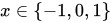
Consider the function $f(x)=x^{8}+1$. Evaluating the function and its first two derivatives at $x\in \{-1,0,1\}$, we obtain the following data:

x	f(x)	f′(x)	f″(x)
−1	2	−8	56
0	1	0	0
1	2	8	56

Since we have two derivatives to work with, we construct the set $\{z_{i}\}=\{-1,-1,-1,0,0,0,1,1,1\}$. Our divided difference table is then: $${\begin{array}{llcclrrrrr}z_{0}=-1&f[z_{0}]=2&&&&&&&&\\&&{\frac {f'(z_{0})}{1}}=-8&&&&&&&\\z_{1}=-1&f[z_{1}]=2&&{\frac {f''(z_{1})}{2}}=28&&&&&&\\&&{\frac {f'(z_{1})}{1}}=-8&&f[z_{3},z_{2},z_{1},z_{0}]=-21&&&&&\\z_{2}=-1&f[z_{2}]=2&&f[z_{3},z_{2},z_{1}]=7&&15&&&&\\&&f[z_{3},z_{2}]=-1&&f[z_{4},z_{3},z_{2},z_{1}]=-6&&-10&&&\\z_{3}=0&f[z_{3}]=1&&f[z_{4},z_{3},z_{2}]=1&&5&&4&&\\&&{\frac {f'(z_{3})}{1}}=0&&f[z_{5},z_{4},z_{3},z_{2}]=-1&&-2&&-1&\\z_{4}=0&f[z_{4}]=1&&{\frac {f''(z_{4})}{2}}=0&&1&&2&&1\\&&{\frac {f'(z_{4})}{1}}=0&&f[z_{6},z_{5},z_{4},z_{3}]=1&&2&&1&\\z_{5}=0&f[z_{5}]=1&&f[z_{6},z_{5},z_{4}]=1&&5&&4&&\\&&f[z_{6},z_{5}]=1&&f[z_{7},z_{6},z_{5},z_{4}]=6&&10&&&\\z_{6}=1&f[z_{6}]=2&&f[z_{7},z_{6},z_{5}]=7&&15&&&&\\&&{\frac {f'(z_{6})}{1}}=8&&f[z_{8},z_{7},z_{6},z_{5}]=21&&&&&\\z_{7}=1&f[z_{7}]=2&&{\frac {f''(z_{7})}{2}}=28&&&&&&\\&&{\frac {f'(z_{7})}{1}}=8&&&&&&&\\z_{8}=1&f[z_{8}]=2&&&&&&&&\\\end{array}}$$ and the generated polynomial is $${\begin{aligned}P(x)&=2-8(x+1)+28(x+1)^{2}-21(x+1)^{3}+15x(x+1)^{3}-10x^{2}(x+1)^{3}\\&\quad {}+4x^{3}(x+1)^{3}-1x^{3}(x+1)^{3}(x-1)+x^{3}(x+1)^{3}(x-1)^{2}\\&=2-8+28-21-8x+56x-63x+15x+28x^{2}-63x^{2}+45x^{2}-10x^{2}-21x^{3}\\&\quad {}+45x^{3}-30x^{3}+4x^{3}+x^{3}+x^{3}+15x^{4}-30x^{4}+12x^{4}+2x^{4}+x^{4}\\&\quad {}-10x^{5}+12x^{5}-2x^{5}+4x^{5}-2x^{5}-2x^{5}-x^{6}+x^{6}-x^{7}+x^{7}+x^{8}\\&=x^{8}+1.\end{aligned}}$$ by taking the coefficients from the diagonal of the divided difference table, and multiplying the kth coefficient by ${\textstyle \prod _{i=0}^{k-1}(x-z_{i})}$, as we would when generating a Newton polynomial.

Quintic Hermite interpolation

The quintic Hermite interpolation based on the function ($f$), its first ($f'$) and second derivatives ($f''$) at two different points ($x_{0}$ and $x_{1}$) can be used for example to interpolate the position of an object based on its position, velocity and acceleration. The general form is given by $${\begin{aligned}p(x)&=f(x_{0})+f'(x_{0})(x-x_{0})+{\frac {1}{2}}f''(x_{0})(x-x_{0})^{2}+{\frac {f(x_{1})-f(x_{0})-f'(x_{0})(x_{1}-x_{0})-{\frac {1}{2}}f''(x_{0})(x_{1}-x_{0})^{2}}{(x_{1}-x_{0})^{3}}}(x-x_{0})^{3}\\&+{\frac {3f(x_{0})-3f(x_{1})+2\left(f'(x_{0})+{\frac {1}{2}}f'(x_{1})\right)(x_{1}-x_{0})+{\frac {1}{2}}f''(x_{0})(x_{1}-x_{0})^{2}}{(x_{1}-x_{0})^{4}}}(x-x_{0})^{3}(x-x_{1})\\&+{\frac {6f(x_{1})-6f(x_{0})-3\left(f'(x_{0})+f'(x_{1})\right)(x_{1}-x_{0})+{\frac {1}{2}}\left(f''(x_{1})-f''(x_{0})\right)(x_{1}-x_{0})^{2}}{(x_{1}-x_{0})^{5}}}(x-x_{0})^{3}(x-x_{1})^{2}.\end{aligned}}$$

A perspective from linear algebra

See also: Vandermonde matrix § Confluent Vandermonde matrices, and Lagrange polynomial § A perspective from linear algebra

The interpolation problem can also be formulated and solved directly using linear algebra in a similar way to Lagrange interpolation, by replacing the standard Vandermonde matrix with a confluent Vandermonde matrix to account for both function values and derivative conditions at each node.

Let k be the number of distinct nodes ${\textstyle x_{1},\ldots ,x_{k}}$, let ${\textstyle n_{i}}$ be the multiplicity of node ${\textstyle x_{i}}$ representing the number of specified values including derivatives, and let ${\textstyle n=\sum _{i=1}^{k}n_{i}}$ be the total number of data conditions. Let V be the confluent Vandermonde matrix, let ${\textstyle H=V^{-1}}$ be its inverse, and let ${\textstyle d=n-1}$ be the degree bound of the interpolating polynomial. The matrix H is given by:

$$H={\begin{pmatrix}H_{00}&\cdots &H_{0d}\\\vdots &\ddots &\vdots \\H_{d0}&\cdots &H_{dd}\end{pmatrix}}.$$

The sample vector ${\textstyle \mathbf {y} }$ stacks all target function values and derivative constraints into a single column vector of total dimension n. The pair of node index i and derivative index j is mapped to a single flattened index ${\textstyle m\in \{0,\dots ,d\}}$ via the indexing function:

$$m=\sigma (i,j)=j+\sum _{l=1}^{i-1}n_{l}.$$

Given the sample vector ${\textstyle \mathbf {y} }$, the coefficient vector ${\textstyle \mathbf {a} ={\begin{pmatrix}a_{0}&a_{1}&\cdots &a_{d}\end{pmatrix}}^{T}}$ of the Hermite interpolating polynomial ${\textstyle f(x)=\sum _{l=0}^{d}a_{l}x^{l}}$ can be computed as:

$$\mathbf {a} =H\mathbf {y} .$$

Furthermore, the individual Hermite interpolating basis polynomials ${\textstyle f_{i,j}(x)}$ correspond to the basis polynomials ${\textstyle h_{m}(x)}$ in the flattened indexing under ${\textstyle m=\sigma (i,j)}$, allowing the interpolating polynomial to be expressed equivalently as:

$$f(x)=\sum _{l=0}^{d}y_{l}h_{l}(x)=\sum _{i=1}^{k}\sum _{j=0}^{n_{i}-1}y_{\sigma (i,j)}f_{i,j}(x).$$

The basis polynomials ${\textstyle f_{i,j}(x)=h_{m}(x)}$ can be constructed directly from the columns of H:

$$f_{i,j}(x)=h_{m}(x)=H_{0m}+H_{1m}x+\cdots +H_{dm}x^{d}.$$

In numerical practice, directly computing H by inverting the confluent Vandermonde matrix is generally avoided because confluent Vandermonde matrices are notoriously ill-conditioned. As the number of nodes or their degree increases, their condition number grows exponentially, making direct matrix inversion numerically unstable and highly sensitive to floating-point errors.

Basis polynomials

For a given set of k distinct nodes ${\textstyle x_{1},\dots ,x_{k}}$ with associated maximum derivative orders ${\textstyle m_{1},\dots ,m_{k}}$, let ${\textstyle n_{i}=m_{i}+1}$ be the multiplicity of node ${\textstyle x_{i}}$, and let ${\textstyle n=\sum _{i}n_{i}}$ be the total number of conditions. The Hermite interpolating polynomial ${\textstyle f(x)}$ can be expressed as a linear combination of basis polynomials ${\textstyle f_{i,j}(x)}$:

$$f(x)=\sum _{i}\sum _{j=0}^{m_{i}}y_{i,j}f_{i,j}(x),$$

where each basis polynomial ${\textstyle f_{i,j}(x)}$ is uniquely defined as the interpolating polynomial of degree at most ${\textstyle n-1}$ for the dual basis conditions given by the Kronecker delta:

$$\left.{\frac {d^{l}}{dx^{l}}}f_{i,j}(x)\right|_{x=x_{r}}=\delta _{i,r}\delta _{j,l}={\begin{cases}1&{\text{if }}r=i{\text{ and }}l=j,\\0&{\text{otherwise.}}\end{cases}}$$

To construct a specific basis polynomial ${\textstyle f_{i,j}(x)}$ using general methods for solving Hermite interpolation (such as those described in this article), one specifies a system of target conditions ${\textstyle y_{r,l}^{(i,j)}}$ across all nodes ${\textstyle x_{r}}$ and derivative orders ${\textstyle 0\leq l\leq m_{r}}$:

$$y_{r,l}^{(i,j)}=\delta _{i,r}\delta _{j,l}={\begin{cases}1&{\text{if }}r=i{\text{ and }}l=j,\\0&{\text{otherwise.}}\end{cases}}$$

By passing these target conditions ${\textstyle y_{r,l}^{(i,j)}}$ as input values into any general method for solving Hermite interpolation, the resulting unique interpolating polynomial generated by the method is precisely the basis polynomial ${\textstyle f_{i,j}(x)}$. Repeating this process for each pair of indices (${\textstyle i,j}$) constructs the full set of n basis polynomials.

Alternative basis construction via degree-0 basis polynomials

Let ${\textstyle q(x)=\prod _{i}(x-x_{i})^{n_{i}}}$ be the polynomial of degree n, which vanishes at each node ${\textstyle x_{i}}$ with multiplicity ${\textstyle n_{i}}$. Once the degree-0 basis polynomials ${\textstyle f_{i,0}(x)}$ (corresponding to the function value condition ${\textstyle y_{i,0}=1}$ at node ${\textstyle x_{i}}$) are obtained, the higher-order derivative basis polynomials ${\textstyle f_{i,j}(x)}$ for ${\textstyle 1\leq j\leq m_{i}}$ can be constructed directly via polynomial reduction:

$$f_{i,j}(x)=\left({\frac {(x-x_{i})^{j}}{j!}}f_{i,0}(x)\right){\bmod {q}}(x).$$

Taking the remainder modulo ${\textstyle q(x)}$ guarantees that ${\textstyle \deg(f_{i,j})<\deg(q)=n}$, projecting the polynomial into the subspace of degree at most ${\textstyle n-1}$. Because ${\textstyle q(x)}$ vanishes at every node ${\textstyle x_{i}}$ to order ${\textstyle n_{i}}$, all target derivative evaluation conditions at the nodes are preserved under this modular reduction. This bounds the degree and ensures that each constructed ${\textstyle f_{i,j}(x)}$ is the unique polynomial of degree at most ${\textstyle n-1}$ satisfying its corresponding interpolation conditions.

This construction is particularly advantageous when direct evaluation of higher-order basis polynomials ${\textstyle f_{i,j}(x)}$ is computationally expensive or numerically unstable. In some cases, the degree-0 basis polynomials ${\textstyle f_{i,0}(x)}$ are simply cleaner and easier to construct and compute, allowing all remaining derivative basis polynomials for that node to be generated efficiently through straightforward polynomial multiplication and modular reduction.

Error

Let k be the number of distinct nodes ${\textstyle x_{1},\ldots ,x_{k}}$, let ${\textstyle n_{i}}$ be the multiplicity of node ${\textstyle x_{i}}$ representing the number of specified values including derivatives, and let ${\textstyle n=\sum _{i=1}^{k}n_{i}}$ be the total number of data conditions. Call the calculated polynomial f and original function y. Consider first the real-valued case. Without loss of generality, assume the nodes are ordered such that ${\textstyle x_{1}<x_{2}<\cdots <x_{k}}$ (since permuting the nodes yields the same interpolating polynomial). Evaluating at a point ${\textstyle x\in [x_{1},x_{k}]}$, the error function is $$y(x)-f(x)={\frac {y^{(n)}(c)}{n!}}\prod _{i=1}^{k}(x-x_{i})^{n_{i}},$$ where c is an unknown value within the range ${\textstyle [x_{1},x_{k}]}$. The degree of the product polynomial on the right is n, which is one higher than the degree bound ${\textstyle n-1}$ for ${\textstyle f(x)}$. Furthermore, the error and all its derivatives up to order ${\textstyle n_{i}-1}$ are zero at each node ${\textstyle x_{i}}$, as expected.

In the complex case, as described for example on p. 360 in , $$y(z)-f(z)={\frac {q(z)}{2\pi i}}\oint _{C}{\frac {y(\zeta )}{q(\zeta )(\zeta -z)}}d\zeta$$ where the contour C encloses z and all the nodes ${\textstyle x_{i}}$, and ${\textstyle q(z)=\prod _{i=1}^{k}(z-x_{i})^{n_{i}}}$ is the product polynomial of all node factors.

See also

• Cubic Hermite spline
• Newton series, also known as finite differences
• Neville's schema
• Bernstein polynomials

External links

• Hermites Interpolating Polynomial at Mathworld