// Workers AI · dad joke modeWhat did Girsanov theorem say to math? "You can't change my measure-ment.

Visualisation of the Girsanov theorem. The left side shows a Wiener process with negative drift under a canonical measure P; on the right side each path of the process is colored according to its likelihood under the martingale measure Q. The density transformation from P to Q is given by the Girsanov theorem.

In probability theory, Girsanov's theorem or the Cameron-Martin-Girsanov theorem explains how stochastic processes change under changes in measure. The theorem is especially important in the theory of financial mathematics as it explains how to convert from the physical measure, which describes the probability that an underlying instrument (such as a share price or interest rate) will take a particular value or values, to the risk-neutral measure which is a very useful tool for evaluating the value of derivatives on the underlying instrument.

History

Results of this type were first proved by Robert Horton Cameron and W. T. Martin in the 1940s and by Igor Girsanov in 1960. They have been subsequently extended to more general classes of process culminating in the general form of Érik Lenglart (1977).

Significance

Girsanov's theorem is important in the general theory of stochastic processes since it enables the key result that if Q is a measure that is absolutely continuous with respect to P then every P-semimartingale is a Q-semimartingale.

Statement of theorem

We state the theorem first for the special case when the underlying stochastic process is a Wiener process. This special case is sufficient for risk-neutral pricing in the Black–Scholes model.

Let $\{W_{t}\}$ be a Wiener process on the Wiener probability space $\{\Omega ,{\mathcal {F}},P\}$. Let $X_{t}$ be a measurable process adapted to the natural filtration of the Wiener process $\{{\mathcal {F}}_{t}^{W}\}$; we assume that the usual conditions have been satisfied.

Given an adapted process $X_{t}$ define

$Z_{t}={\mathcal {E}}(X)_{t},\,$

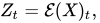
where ${\mathcal {E}}(X)$ is the stochastic exponential of X with respect to W, i.e.

${\mathcal {E}}(X)_{t}=\exp \left(X_{t}-{\frac {1}{2}}[X]_{t}\right),$

and $[X]_{t}$ denotes the quadratic variation of the process X.

If $Z_{t}$ is a martingale then a probability measure Q can be defined on $\{\Omega ,{\mathcal {F}}\}$ such that the Radon–Nikodym derivative of Q with respect to P satisfies

$\left.{\frac {dQ}{dP}}\right|_{{\mathcal {F}}_{t}}=Z_{t}={\mathcal {E}}(X)_{t}$.

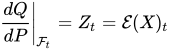
Then for each t the measure Q restricted to the unaugmented sigma fields ${\mathcal {F}}_{t}^{o}$ is equivalent to P restricted to

${\mathcal {F}}_{t}^{o}.\,$

Furthermore, if $Y_{t}$ is a local martingale under P then the process

${\tilde {Y}}_{t}=Y_{t}-\left[Y,X\right]_{t}$

is a Q local martingale on the filtered probability space $\{\Omega ,F,Q,\{{\mathcal {F}}_{t}^{W}\}\}$.

Corollary

If X is a continuous process and W is a Brownian motion under measure P then

${\tilde {W}}_{t}=W_{t}-\left[W,X\right]_{t}$

is a Brownian motion under Q.

The fact that ${\tilde {W}}_{t}$ is continuous is trivial; by Girsanov's theorem it is a Q local martingale, and by computing

$\left[{\tilde {W}}\right]_{t}=\left[W\right]_{t}=t$

it follows by Levy's characterization of Brownian motion that this is a Q Brownian motion.

Comments

In many common applications, the process X is defined by

$X_{t}=\int _{0}^{t}Y_{s}\,dW_{s}.$

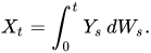
For X of this form then a necessary and sufficient condition for ${\mathcal {E}}(X)$ to be a martingale is Novikov's condition which requires that

$E_{P}\left[\exp \left({\frac {1}{2}}\int _{0}^{T}Y_{s}^{2}\,ds\right)\right]<\infty .$

The stochastic exponential ${\mathcal {E}}(X)$ is the process Z which solves the stochastic differential equation

$Z_{t}=1+\int _{0}^{t}Z_{s}\,dX_{s}.\,$

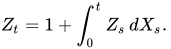
The measure Q constructed above is not equivalent to P on ${\mathcal {F}}_{\infty }$ as this would only be the case if the Radon–Nikodym derivative were a uniformly integrable martingale, which the exponential martingale described above is not. On the other hand, as long as Novikov's condition is satisfied the measures are equivalent on ${\mathcal {F}}_{T}$.

Additionally, then combining this above observation in this case, we see that the process

${\tilde {W}}_{t}=W_{t}-\int _{0}^{t}Y_{s}ds$

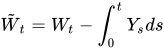
for $t\in [0,T]$ is a Q Brownian motion. This was Igor Girsanov's original formulation of the above theorem.

Application to finance

Consider a non-dividend-paying risky asset whose price under the physical measure $P$ follows the stochastic differential equation

${\frac {dS_{t}}{S_{t}}}=\mu _{t}\,dt+\sigma _{t}\,dW_{t}^{P},\qquad \sigma _{t}>0,$

where $\mu _{t}$ is the asset's drift, $\sigma _{t}$ is its instantaneous volatility, and $W^{P}$ is a Brownian motion under $P$. Let

$\lambda _{t}={\frac {\mu _{t}-r_{t}}{\sigma _{t}}},$

where $r_{t}$ is the risk-free rate, and suppose that the associated stochastic exponential is a martingale. Define a new probability measure $Q$ by

$\left.{\frac {dQ}{dP}}\right|_{{\mathcal {F}}_{t}}={\mathcal {E}}\left(-\int _{0}^{t}\lambda _{s}\,dW_{s}^{P}\right).$

Girsanov's theorem then implies that

$W_{t}^{Q}=W_{t}^{P}+\int _{0}^{t}\lambda _{s}\,ds$

is a Brownian motion under $Q$. Substitution into the asset-price equation gives

${\frac {dS_{t}}{S_{t}}}=r_{t}\,dt+\sigma _{t}\,dW_{t}^{Q}.$

Thus, the change from the physical measure to the risk-neutral measure changes the asset's drift from $\mu _{t}$ to the risk-free rate $r_{t}$, while leaving the diffusion coefficient $\sigma _{t}$, or instantaneous volatility, unchanged.

This invariance concerns the diffusion coefficient within a specified model. It does not imply that estimates of historical volatility and implied volatility must be equal; those estimates may differ in practice.

Under $Q$, the discounted asset-price process is a martingale. In an arbitrage-free and complete market, such as the Black–Scholes-Merton model, the risk-neutral measure is unique, and the value at time $t$ of a contingent claim paying $H_{T}$ at time $T$ is

$V_{t}=E_{Q}\left[\left.\exp \left(-\int _{t}^{T}r_{s}\,ds\right)H_{T}\right|{\mathcal {F}}_{t}\right].$

Girsanov's theorem provides the change of measure, while the uniqueness of the measure and the valuation formula depend on the model's no-arbitrage and completeness assumptions.

Application to Langevin equations

Another application of this theorem, also given in the original paper of Igor Girsanov, is for stochastic differential equations. Specifically, let us consider the equation:

$dX_{t}=\mu (X_{t},t)dt+\sigma (X_{t},t)dW_{t}.$

where $W_{t}$ denotes a Brownian motion. Here $\mu$ and $\sigma$ are fixed deterministic functions. We assume that this equation has a unique strong solution on $[0,T]$. In this case Girsanov's theorem may be used to compute functionals of $X_{t}$ directly in terms a related functional for Brownian motion. More specifically, we have for any bounded functional $\Phi$ on continuous functions $C([0,T])$ that

$E\Phi (X)=E\left[\Phi (W)\exp \left(\int _{0}^{T}\mu (W_{s},s)dW_{s}-{\frac {1}{2}}\int _{0}^{T}\mu (W_{s},s)^{2}ds\right)\right].$

This follows by applying Girsanov's theorem, and the above observation, to the martingale process

$Y_{t}=\int _{0}^{t}\mu (W_{s},s)dW_{s}.$

In particular, with the notation above, the process

${\tilde {W}}_{t}=W_{t}-\int _{0}^{t}\mu (W_{s},s)ds$

is a Q Brownian motion. Rewriting this in differential notation as

$dW_{t}=d{\tilde {W}}_{t}+\mu (W_{t},t)dt,$

we see that the law of $W_{t}$ under Q solves the equation defining $X_{t}$, as ${\tilde {W}}_{t}$ is a Q Brownian motion. In particular, we see that the right-hand side may be written as $E_{Q}[\Phi (W)]$, where Q is the measure taken with respect to the process Y, so the result now is just the statement of Girsanov's theorem.

A more general form of this application is that if both

$dX_{t}=\mu (X_{t},t)dt+\sigma (X_{t},t)dW_{t},$ $dY_{t}=(\mu (Y_{t},t)+\nu (Y_{t},t))dt+\sigma (Y_{t},t)dW_{t},$

admit unique strong solutions on $[0,T]$, then for any bounded functional on $C([0,T])$, we have that

$E\Phi (X)=E\left[\Phi (Y)\exp \left(-\int _{0}^{T}{\frac {\nu (Y_{s},s)}{\sigma (Y_{s},s)}}dW_{s}-{\frac {1}{2}}\int _{0}^{T}{\frac {\nu (Y_{s},s)^{2}}{\sigma (Y_{s},s)^{2}}}ds\right)\right].$

See also

• Cameron–Martin theorem – Theorem describing translation of Gaussian measures on Hilbert spaces It is a special case of the Girsanov theorem who has inspired all the theory.
• Girsanov theorem has fundamental applications to the Quantum Field Theory, Malliavin Calculus, stochastic partial differential equations, degree theory, calculus of variations on the classical and abstract Wiener spaces.

References

• Liptser, Robert S.; Shiriaev, A. N. (2001). Statistics of Random Processes (2nd, rev. and exp. ed.). Springer. ISBN 3-540-63929-2.
• Dellacherie, C.; Meyer, P.-A. (1982). "Decomposition of Supermartingales, Applications". Probabilities and Potential. Vol. B. Translated by Wilson, J. P. North-Holland. pp. 183–308. ISBN 0-444-86526-8.
• Lenglart, E. (1977). "Transformation de martingales locales par changement absolue continu de probabilités". Zeitschrift für Wahrscheinlichkeit (in French). 39: 65–70. doi:10.1007/BF01844873.
• \"Ust\"unel, A. S.; Zakai, M. (2000). Transformation of Measure on Wiener space (1st ed.). Springer. ISBN 3-540-66455-6.

External links

• Notes on Stochastic Calculus which contain a simple outline proof of Girsanov's theorem.

References

[edit]- ↑ Desmettre, Sascha; Leobacher, Gunther; Rogers, L. C. G. (2021). "Change of drift in one-dimensional diffusions". Finance and Stochastics. 25: 359–381. arXiv:1910.11904. doi:10.1007/s00780-021-00451-w.
- 1 2 Hull, John; Sokol, Alexander; White, Alan (October 2014). "Short Rate Joint Measure Models" (PDF). Risk: 59–63. Retrieved 25 July 2026.
- ↑ Harrison, J. Michael; Pliska, Stanley R. (1981). "Martingales and stochastic integrals in the theory of continuous trading". Stochastic Processes and their Applications. 11 (3): 215–260. doi:10.1016/0304-4149(81)90026-0.
- ↑ Black, Fischer; Scholes, Myron (1973). "The Pricing of Options and Corporate Liabilities". Journal of Political Economy. 81 (3): 637–654. doi:10.1086/260062.