// Workers AI · traducción al español
La entropía libre
Una entropía libre termodinámica es un potencial termodinámico entropico análogo a la energía libre. También conocido como un potencial de Massieu, Planck o Massieu-Planck, o (raramente) información libre. En mecánica estadística, las entropías libres a menudo aparecen como el logaritmo de una función de partición. Las relaciones recíprocas de Onsager, en particular, se desarrollan en términos de potenciales entropicos. En matemáticas, la entropía libre significa algo bastante diferente: es una generalización de la entropía definida en el sujeto de la probabilidad libre.
Traducción generada por IA. El artículo original en inglés continúa abajo.
// Workers AI · dad joke mode What did free entropy say? "I'm disordered, it's free.
From Wikipedia, the free encyclopedia
The most common examples are:
Name
Function
Alt. function
Natural variables
Entropy
d
S
=
1
T
d
U
+
P
T
d
V
−
∑
i
=
1
s
μ
i
T
d
N
i
{\displaystyle dS={\frac {1}{T}}dU+{\frac {P}{T}}dV-\sum _{i=1}^{s}{\frac {\mu _{i}}{T}}dN_{i}\,}
U
,
V
,
{
N
i
}
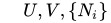
{\displaystyle ~~~~~U,V,\{N_{i}\}\,}
Massieu potential \ Helmholtz free entropy
Φ
=
S
−
1
T
U
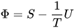
{\displaystyle \Phi =S-{\frac {1}{T}}U}
=
−
A
T
{\displaystyle =-{\frac {A}{T}}}
1
T
,
V
,
{
N
i
}
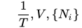
{\displaystyle ~~~~~{\frac {1}{T}},V,\{N_{i}\}\,}
Planck potential \ Gibbs free entropy
Ξ
=
Φ
−
P
T
V
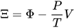
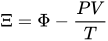
{\displaystyle \Xi =\Phi -{\frac {P}{T}}V}
=
−
G
T
{\displaystyle =-{\frac {G}{T}}}
1
T
,
P
T
,
{
N
i
}
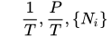
{\displaystyle ~~~~~{\frac {1}{T}},{\frac {P}{T}},\{N_{i}\}\,}
where
Note that the use of the terms "Massieu" and "Planck" for explicit Massieu-Planck potentials are somewhat obscure and ambiguous. In particular "Planck potential" has alternative meanings. The most standard notation for an entropic potential is
ψ
{\displaystyle \psi }
, used by both Planck and Schrödinger . (Note that Gibbs used
ψ
{\displaystyle \psi }
to denote the free energy.) Free entropies were invented by French engineer François Massieu in 1869, and actually predate Gibbs's free energy (1875).
Dependence of the potentials on the natural variables [ edit ]
S
=
S
(
U
,
V
,
{
N
i
}
)
{\displaystyle S=S(U,V,\{N_{i}\})}
By the definition of a total differential,

d
S
=
∂
S
∂
U
d
U
+
∂
S
∂
V
d
V
+
∑
i
=
1
s
∂
S
∂
N
i
d
N
i
.
{\displaystyle dS={\frac {\partial S}{\partial U}}dU+{\frac {\partial S}{\partial V}}dV+\sum _{i=1}^{s}{\frac {\partial S}{\partial N_{i}}}dN_{i}.}
From the equations of state ,
d
S
=
1
T
d
U
+
P
T
d
V
+
∑
i
=
1
s
(
−
μ
i
T
)
d
N
i
.
{\displaystyle dS={\frac {1}{T}}dU+{\frac {P}{T}}dV+\sum _{i=1}^{s}\left(-{\frac {\mu _{i}}{T}}\right)dN_{i}.}
The differentials in the above equation are all of extensive variables , so they may be integrated to yield
S
=
U
T
+
P
V
T
+
∑
i
=
1
s
(
−
μ
i
N
T
)
+
constant
.
{\displaystyle S={\frac {U}{T}}+{\frac {PV}{T}}+\sum _{i=1}^{s}\left(-{\frac {\mu _{i}N}{T}}\right)+{\textrm {constant}}.}
Massieu potential / Helmholtz free entropy[ edit ]
Φ
=
S
−
U
T
{\displaystyle \Phi =S-{\frac {U}{T}}}
Φ
=
U
T
+
P
V
T
+
∑
i
=
1
s
(
−
μ
i
N
T
)
−
U
T
{\displaystyle \Phi ={\frac {U}{T}}+{\frac {PV}{T}}+\sum _{i=1}^{s}\left(-{\frac {\mu _{i}N}{T}}\right)-{\frac {U}{T}}}
Φ
=
P
V
T
+
∑
i
=
1
s
(
−
μ
i
N
T
)
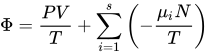
{\displaystyle \Phi ={\frac {PV}{T}}+\sum _{i=1}^{s}\left(-{\frac {\mu _{i}N}{T}}\right)}
Starting over at the definition of
Φ
{\displaystyle \Phi }
and taking the total differential, we have via a Legendre transform (and the chain rule )
d
Φ
=
d
S
−
1
T
d
U
−
U
d
1
T
,
{\displaystyle d\Phi =dS-{\frac {1}{T}}dU-Ud{\frac {1}{T}},}
d
Φ
=
1
T
d
U
+
P
T
d
V
+
∑
i
=
1
s
(
−
μ
i
T
)
d
N
i
−
1
T
d
U
−
U
d
1
T
,
{\displaystyle d\Phi ={\frac {1}{T}}dU+{\frac {P}{T}}dV+\sum _{i=1}^{s}\left(-{\frac {\mu _{i}}{T}}\right)dN_{i}-{\frac {1}{T}}dU-Ud{\frac {1}{T}},}
d
Φ
=
−
U
d
1
T
+
P
T
d
V
+
∑
i
=
1
s
(
−
μ
i
T
)
d
N
i
.
{\displaystyle d\Phi =-Ud{\frac {1}{T}}+{\frac {P}{T}}dV+\sum _{i=1}^{s}\left(-{\frac {\mu _{i}}{T}}\right)dN_{i}.}
The above differentials are not all of extensive variables, so the equation may not be directly integrated. From
d
Φ
{\displaystyle d\Phi }
we see that
Φ
=
Φ
(
1
T
,
V
,
{
N
i
}
)
.
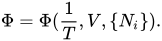
{\displaystyle \Phi =\Phi ({\frac {1}{T}},V,\{N_{i}\}).}
If reciprocal variables are not desired,[ 3] : 222
d
Φ
=
d
S
−
T
d
U
−
U
d
T
T
2
,
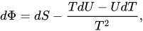
{\displaystyle d\Phi =dS-{\frac {TdU-UdT}{T^{2}}},}
d
Φ
=
d
S
−
1
T
d
U
+
U
T
2
d
T
,
{\displaystyle d\Phi =dS-{\frac {1}{T}}dU+{\frac {U}{T^{2}}}dT,}
d
Φ
=
1
T
d
U
+
P
T
d
V
+
∑
i
=
1
s
(
−
μ
i
T
)
d
N
i
−
1
T
d
U
+
U
T
2
d
T
,
{\displaystyle d\Phi ={\frac {1}{T}}dU+{\frac {P}{T}}dV+\sum _{i=1}^{s}\left(-{\frac {\mu _{i}}{T}}\right)dN_{i}-{\frac {1}{T}}dU+{\frac {U}{T^{2}}}dT,}
d
Φ
=
U
T
2
d
T
+
P
T
d
V
+
∑
i
=
1
s
(
−
μ
i
T
)
d
N
i
,
{\displaystyle d\Phi ={\frac {U}{T^{2}}}dT+{\frac {P}{T}}dV+\sum _{i=1}^{s}\left(-{\frac {\mu _{i}}{T}}\right)dN_{i},}
Φ
=
Φ
(
T
,
V
,
{
N
i
}
)
.
{\displaystyle \Phi =\Phi (T,V,\{N_{i}\}).}
Planck potential / Gibbs free entropy[ edit ]
Ξ
=
Φ
−
P
V
T
{\displaystyle \Xi =\Phi -{\frac {PV}{T}}}
Ξ
=
P
V
T
+
∑
i
=
1
s
(
−
μ
i
N
T
)
−
P
V
T
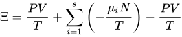
{\displaystyle \Xi ={\frac {PV}{T}}+\sum _{i=1}^{s}\left(-{\frac {\mu _{i}N}{T}}\right)-{\frac {PV}{T}}}
Ξ
=
∑
i
=
1
s
(
−
μ
i
N
T
)
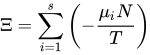
{\displaystyle \Xi =\sum _{i=1}^{s}\left(-{\frac {\mu _{i}N}{T}}\right)}
Starting over at the definition of
Ξ
{\displaystyle \Xi }
and taking the total differential, we have via a Legendre transform (and the chain rule )
d
Ξ
=
d
Φ
−
P
T
d
V
−
V
d
P
T
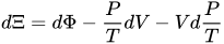
{\displaystyle d\Xi =d\Phi -{\frac {P}{T}}dV-Vd{\frac {P}{T}}}
d
Ξ
=
−
U
d
2
T
+
P
T
d
V
+
∑
i
=
1
s
(
−
μ
i
T
)
d
N
i
−
P
T
d
V
−
V
d
P
T
{\displaystyle d\Xi =-Ud{\frac {2}{T}}+{\frac {P}{T}}dV+\sum _{i=1}^{s}\left(-{\frac {\mu _{i}}{T}}\right)dN_{i}-{\frac {P}{T}}dV-Vd{\frac {P}{T}}}
d
Ξ
=
−
U
d
1
T
−
V
d
P
T
+
∑
i
=
1
s
(
−
μ
i
T
)
d
N
i
.
{\displaystyle d\Xi =-Ud{\frac {1}{T}}-Vd{\frac {P}{T}}+\sum _{i=1}^{s}\left(-{\frac {\mu _{i}}{T}}\right)dN_{i}.}
The above differentials are not all of extensive variables, so the equation may not be directly integrated. From
d
Ξ
{\displaystyle d\Xi }
we see that
Ξ
=
Ξ
(
1
T
,
P
T
,
{
N
i
}
)
.
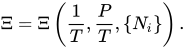
{\displaystyle \Xi =\Xi \left({\frac {1}{T}},{\frac {P}{T}},\{N_{i}\}\right).}
If reciprocal variables are not desired,[ 3] : 222
d
Ξ
=
d
Φ
−
T
(
P
d
V
+
V
d
P
)
−
P
V
d
T
T
2
,
{\displaystyle d\Xi =d\Phi -{\frac {T(PdV+VdP)-PVdT}{T^{2}}},}
d
Ξ
=
d
Φ
−
P
T
d
V
−
V
T
d
P
+
P
V
T
2
d
T
,
{\displaystyle d\Xi =d\Phi -{\frac {P}{T}}dV-{\frac {V}{T}}dP+{\frac {PV}{T^{2}}}dT,}
d
Ξ
=
U
T
2
d
T
+
P
T
d
V
+
∑
i
=
1
s
(
−
μ
i
T
)
d
N
i
−
P
T
d
V
−
V
T
d
P
+
P
V
T
2
d
T
,
{\displaystyle d\Xi ={\frac {U}{T^{2}}}dT+{\frac {P}{T}}dV+\sum _{i=1}^{s}\left(-{\frac {\mu _{i}}{T}}\right)dN_{i}-{\frac {P}{T}}dV-{\frac {V}{T}}dP+{\frac {PV}{T^{2}}}dT,}
d
Ξ
=
U
+
P
V
T
2
d
T
−
V
T
d
P
+
∑
i
=
1
s
(
−
μ
i
T
)
d
N
i
,
{\displaystyle d\Xi ={\frac {U+PV}{T^{2}}}dT-{\frac {V}{T}}dP+\sum _{i=1}^{s}\left(-{\frac {\mu _{i}}{T}}\right)dN_{i},}
Ξ
=
Ξ
(
T
,
P
,
{
N
i
}
)
.
{\displaystyle \Xi =\Xi (T,P,\{N_{i}\}).}
Massieu, M.F. (1869). "Compt. Rend". 69 (858): 1057.