From Wikipedia, the free encyclopedia
Special case of the polylogarithm
"Li2" redirects here. For the molecule with formula Li
2 , see
dilithium .
The dilogarithm along the real axis The principal value of the dilogarithm plotted in the complex plane In mathematics , the dilogarithm (or Spence's function ), denoted as Li2 (z ) , is a particular case of the polylogarithm . Two related special functions are referred to as Spence's function, the dilogarithm itself:
Li
2
(
z
)
=
−
∫
0
z
ln
(
1
−
u
)
u
d
u
,
z
∈
C
{\displaystyle \operatorname {Li} _{2}(z)=-\int _{0}^{z}{\ln(1-u) \over u}\,du{\text{, }}z\in \mathbb {C} }
and its reflection.
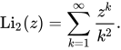
For | z | ≤ 1infinite series also applies (the integral definition constitutes its analytical extension to the complex plane ):
Li
2
(
z
)
=
∑
k
=
1
∞
z
k
k
2
.
{\displaystyle \operatorname {Li} _{2}(z)=\sum _{k=1}^{\infty }{z^{k} \over k^{2}}.}
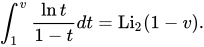
Alternatively, the dilogarithm function is sometimes defined as
∫
1
v
ln
t
1
−
t
d
t
=
Li
2
(
1
−
v
)
.
{\displaystyle \int _{1}^{v}{\frac {\ln t}{1-t}}dt=\operatorname {Li} _{2}(1-v).}
In hyperbolic geometry the dilogarithm can be used to compute the volume of an ideal simplex . Specifically, a simplex whose vertices have cross ratio z has hyperbolic volume
D
(
z
)
=
Im
Li
2
(
z
)
+
arg
(
1
−
z
)
log
|
z
|
.
{\displaystyle D(z)=\operatorname {Im} \operatorname {Li} _{2}(z)+\arg(1-z)\log |z|.}
The function D (z )[ 1] Lobachevsky's function and Clausen's function are closely related functions.
William Spence , after whom the function was named by early writers in the field, was a Scottish mathematician working in the early nineteenth century.[ 2] John Galt ,[ 3]
Li
2
(
z
)
+
Li
2
(
−
z
)
=
1
2
Li
2
(
z
2
)
.
{\displaystyle \operatorname {Li} _{2}(z)+\operatorname {Li} _{2}(-z)={\frac {1}{2}}\operatorname {Li} _{2}(z^{2}).}
[ 4]
Li
2
(
1
−
z
)
+
Li
2
(
1
−
1
z
)
=
−
(
ln
z
)
2
2
.
{\displaystyle \operatorname {Li} _{2}(1-z)+\operatorname {Li} _{2}\left(1-{\frac {1}{z}}\right)=-{\frac {(\ln z)^{2}}{2}}.}
[ 5]
Li
2
(
z
)
+
Li
2
(
1
−
z
)
=
π
2
6
−
ln
z
⋅
ln
(
1
−
z
)
.
{\displaystyle \operatorname {Li} _{2}(z)+\operatorname {Li} _{2}(1-z)={\frac {{\pi }^{2}}{6}}-\ln z\cdot \ln(1-z).}
[ 4] reflection formula .
Li
2
(
−
z
)
−
Li
2
(
1
−
z
)
+
1
2
Li
2
(
1
−
z
2
)
=
−
π
2
12
−
ln
z
⋅
ln
(
z
+
1
)
.
{\displaystyle \operatorname {Li} _{2}(-z)-\operatorname {Li} _{2}(1-z)+{\frac {1}{2}}\operatorname {Li} _{2}(1-z^{2})=-{\frac {{\pi }^{2}}{12}}-\ln z\cdot \ln(z+1).}
[ 5]
Li
2
(
z
)
+
Li
2
(
1
z
)
=
−
π
2
6
−
(
ln
(
−
z
)
)
2
2
.
{\displaystyle \operatorname {Li} _{2}(z)+\operatorname {Li} _{2}\left({\frac {1}{z}}\right)=-{\frac {\pi ^{2}}{6}}-{\frac {(\ln(-z))^{2}}{2}}.}
[ 4]
L
(
x
)
+
L
(
y
)
=
L
(
x
y
)
+
L
(
x
(
1
−
y
)
1
−
x
y
)
+
L
(
y
(
1
−
x
)
1
−
x
y
)
{\displaystyle \operatorname {L} (x)+\operatorname {L} (y)=\operatorname {L} (xy)+\operatorname {L} \left({\frac {x(1-y)}{1-xy}}\right)+\operatorname {L} \left({\frac {y(1-x)}{1-xy}}\right)}
[ 6] [ 7]
L
(
z
)
=
π
2
6
[
Li
2
(
z
)
+
1
2
ln
(
z
)
ln
(
1
−
z
)
]
{\displaystyle \operatorname {L} (z)={\frac {\pi ^{2}}{6}}[\operatorname {Li} _{2}(z)+{\frac {1}{2}}\ln(z)\ln(1-z)]}
Rogers L-function (an analogous relation is satisfied also by the quantum dilogarithm ) Particular value identities [ edit ]
Li
2
(
1
3
)
−
1
6
Li
2
(
1
9
)
=
π
2
18
−
(
ln
3
)
2
6
.
{\displaystyle \operatorname {Li} _{2}\left({\frac {1}{3}}\right)-{\frac {1}{6}}\operatorname {Li} _{2}\left({\frac {1}{9}}\right)={\frac {{\pi }^{2}}{18}}-{\frac {(\ln 3)^{2}}{6}}.}
[ 5]
Li
2
(
−
1
3
)
−
1
3
Li
2
(
1
9
)
=
−
π
2
18
+
(
ln
3
)
2
6
.
{\displaystyle \operatorname {Li} _{2}\left(-{\frac {1}{3}}\right)-{\frac {1}{3}}\operatorname {Li} _{2}\left({\frac {1}{9}}\right)=-{\frac {{\pi }^{2}}{18}}+{\frac {(\ln 3)^{2}}{6}}.}
[ 5]
Li
2
(
−
1
2
)
+
1
6
Li
2
(
1
9
)
=
−
π
2
18
+
ln
2
⋅
ln
3
−
(
ln
2
)
2
2
−
(
ln
3
)
2
3
.
{\displaystyle \operatorname {Li} _{2}\left(-{\frac {1}{2}}\right)+{\frac {1}{6}}\operatorname {Li} _{2}\left({\frac {1}{9}}\right)=-{\frac {{\pi }^{2}}{18}}+\ln 2\cdot \ln 3-{\frac {(\ln 2)^{2}}{2}}-{\frac {(\ln 3)^{2}}{3}}.}
[ 5]
Li
2
(
1
4
)
+
1
3
Li
2
(
1
9
)
=
π
2
18
+
2
ln
2
⋅
ln
3
−
2
(
ln
2
)
2
−
2
3
(
ln
3
)
2
.
{\displaystyle \operatorname {Li} _{2}\left({\frac {1}{4}}\right)+{\frac {1}{3}}\operatorname {Li} _{2}\left({\frac {1}{9}}\right)={\frac {{\pi }^{2}}{18}}+2\ln 2\cdot \ln 3-2(\ln 2)^{2}-{\frac {2}{3}}(\ln 3)^{2}.}
[ 5]
Li
2
(
−
1
8
)
+
Li
2
(
1
9
)
=
−
1
2
(
ln
9
8
)
2
.
{\displaystyle \operatorname {Li} _{2}\left(-{\frac {1}{8}}\right)+\operatorname {Li} _{2}\left({\frac {1}{9}}\right)=-{\frac {1}{2}}\left(\ln {\frac {9}{8}}\right)^{2}.}
[ 5]
36
Li
2
(
1
2
)
−
36
Li
2
(
1
4
)
−
12
Li
2
(
1
8
)
+
6
Li
2
(
1
64
)
=
π
2
.
{\displaystyle 36\operatorname {Li} _{2}\left({\frac {1}{2}}\right)-36\operatorname {Li} _{2}\left({\frac {1}{4}}\right)-12\operatorname {Li} _{2}\left({\frac {1}{8}}\right)+6\operatorname {Li} _{2}\left({\frac {1}{64}}\right)={\pi }^{2}.}
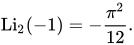
Li
2
(
−
1
)
=
−
π
2
12
.
{\displaystyle \operatorname {Li} _{2}(-1)=-{\frac {{\pi }^{2}}{12}}.}
Li
2
(
0
)
=
0.
{\displaystyle \operatorname {Li} _{2}(0)=0.}
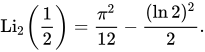
Li
2
(
1
2
)
=
π
2
12
−
(
ln
2
)
2
2
.
{\displaystyle \operatorname {Li} _{2}\left({\frac {1}{2}}\right)={\frac {{\pi }^{2}}{12}}-{\frac {(\ln 2)^{2}}{2}}.}
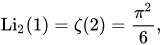
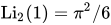
Li
2
(
1
)
=
ζ
(
2
)
=
π
2
6
,
{\displaystyle \operatorname {Li} _{2}(1)=\zeta (2)={\frac {{\pi }^{2}}{6}},}
ζ
(
s
)
{\displaystyle \zeta (s)}
Riemann zeta function .
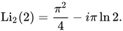
Li
2
(
2
)
=
π
2
4
−
i
π
ln
2.
{\displaystyle \operatorname {Li} _{2}(2)={\frac {{\pi }^{2}}{4}}-i\pi \ln 2.}
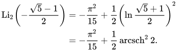
Li
2
(
−
5
−
1
2
)
=
−
π
2
15
+
1
2
(
ln
5
+
1
2
)
2
=
−
π
2
15
+
1
2
arcsch
2
2.
{\displaystyle {\begin{aligned}\operatorname {Li} _{2}\left(-{\frac {{\sqrt {5}}-1}{2}}\right)&=-{\frac {{\pi }^{2}}{15}}+{\frac {1}{2}}\left(\ln {\frac {{\sqrt {5}}+1}{2}}\right)^{2}\\&=-{\frac {{\pi }^{2}}{15}}+{\frac {1}{2}}\operatorname {arcsch} ^{2}2.\end{aligned}}}
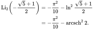
Li
2
(
−
5
+
1
2
)
=
−
π
2
10
−
ln
2
5
+
1
2
=
−
π
2
10
−
arcsch
2
2.
{\displaystyle {\begin{aligned}\operatorname {Li} _{2}\left(-{\frac {{\sqrt {5}}+1}{2}}\right)&=-{\frac {{\pi }^{2}}{10}}-\ln ^{2}{\frac {{\sqrt {5}}+1}{2}}\\&=-{\frac {{\pi }^{2}}{10}}-\operatorname {arcsch} ^{2}2.\end{aligned}}}
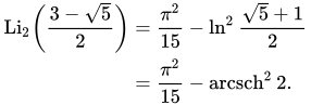
Li
2
(
3
−
5
2
)
=
π
2
15
−
ln
2
5
+
1
2
=
π
2
15
−
arcsch
2
2.
{\displaystyle {\begin{aligned}\operatorname {Li} _{2}\left({\frac {3-{\sqrt {5}}}{2}}\right)&={\frac {{\pi }^{2}}{15}}-\ln ^{2}{\frac {{\sqrt {5}}+1}{2}}\\&={\frac {{\pi }^{2}}{15}}-\operatorname {arcsch} ^{2}2.\end{aligned}}}
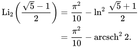
Li
2
(
5
−
1
2
)
=
π
2
10
−
ln
2
5
+
1
2
=
π
2
10
−
arcsch
2
2.
{\displaystyle {\begin{aligned}\operatorname {Li} _{2}\left({\frac {{\sqrt {5}}-1}{2}}\right)&={\frac {{\pi }^{2}}{10}}-\ln ^{2}{\frac {{\sqrt {5}}+1}{2}}\\&={\frac {{\pi }^{2}}{10}}-\operatorname {arcsch} ^{2}2.\end{aligned}}}
In particle physics [ edit ] Spence's Function is commonly encountered in particle physics while calculating radiative corrections . In this context, the function is often defined with an absolute value inside the logarithm:
Φ
(
x
)
=
−
∫
0
x
ln
|
1
−
u
|
u
d
u
=
{
Li
2
(
x
)
,
x
≤
1
;
π
2
3
−
1
2
(
ln
x
)
2
−
Li
2
(
1
x
)
,
x
>
1.
{\displaystyle \operatorname {\Phi } (x)=-\int _{0}^{x}{\frac {\ln |1-u|}{u}}\,du={\begin{cases}\operatorname {Li} _{2}(x),&x\leq 1;\\{\frac {\pi ^{2}}{3}}-{\frac {1}{2}}(\ln x)^{2}-\operatorname {Li} _{2}({\frac {1}{x}}),&x>1.\end{cases}}}
Lewin, L. (1958). Dilogarithms and associated functions . Foreword by J. C. P. Miller. London: Macdonald. MR 0105524 . Morris, Robert (1979). "The dilogarithm function of a real argument" . Math. Comp . 33 (146): 778– 787. doi :10.1090/S0025-5718-1979-0521291-X MR 0521291 . Loxton, J. H. (1984). "Special values of the dilogarithm" . Acta Arith . 18 (2): 155– 166. doi :10.4064/aa-43-2-155-166 MR 0736728 . Kirillov, Anatol N. (1995). "Dilogarithm identities". Progress of Theoretical Physics Supplement . 118 : 61– 142. arXiv :hep-th/9408113 Bibcode :1995PThPS.118...61K . doi :10.1143/PTPS.118.61 . S2CID 119177149 . Osacar, Carlos; Palacian, Jesus; Palacios, Manuel (1995). "Numerical evaluation of the dilogarithm of complex argument". Celest. Mech. Dyn. Astron . 62 (1): 93– 98. Bibcode :1995CeMDA..62...93O . doi :10.1007/BF00692071 . S2CID 121304484 . Zagier, Don (2007). "The Dilogarithm Function". In Pierre Cartier ; Pierre Moussa; Bernard Julia; Pierre Vanhove (eds.). Frontiers in Number Theory, Physics, and Geometry II (PDF) . pp. 3– 65. doi :10.1007/978-3-540-30308-4_1 . ISBN 978-3-540-30308-4












![{\displaystyle \operatorname {L} (z)={\frac {\pi ^{2}}{6}}[\operatorname {Li} _{2}(z)+{\frac {1}{2}}\ln(z)\ln(1-z)]}](https://wikimedia.org/api/rest_v1/media/math/render/svg/dcc3bfc44d20d30ad606b35078a8c720aac97729)