// Workers AI · traducción al español
Descomposición de la varianza de los errores de predicción
En econometría y otras aplicaciones de análisis de serie de tiempo multivariado, una descomposición de varianza o descomposición de varianza de error de predicción (FEVD) se utiliza para ayudar en la interpretación de un modelo de autorregresión vectorial (VAR) una vez que se ha instalado. La descomposición de varianza indica la cantidad de información que cada variable contribuye a las otras variables en la autorregresión. Determina cuánto de la varianza de error de predicción de cada una de las variables se puede explicar por choques exógenos a las otras variables.
Traducción generada por IA. El artículo original en inglés continúa abajo.
Variance decomposition of forecast errors
From Wikipedia, the free encyclopedia
In econometrics and other applications of multivariate time series analysis , a variance decomposition or forecast error variance decomposition (FEVD ) is used to aid in the interpretation of a vector autoregression (VAR) model once it has been fitted.[ 1] variance decomposition indicates the amount of information each variable contributes to the other variables in the autoregression. It determines how much of the forecast error variance of each of the variables can be explained by exogenous shocks to the other variables.
Calculating the forecast error variance [ edit ] For the VAR (p) of form
y
t
=
ν
+
A
1
y
t
−
1
+
⋯
+
A
p
y
t
−
p
+
u
t
{\displaystyle y_{t}=\nu +A_{1}y_{t-1}+\dots +A_{p}y_{t-p}+u_{t}}
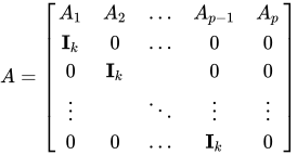
This can be changed to a VAR(1) structure by writing it in companion form (see general matrix notation of a VAR(p))
Y
t
=
V
+
A
Y
t
−
1
+
U
t
{\displaystyle Y_{t}=V+AY_{t-1}+U_{t}}
A
=
[
A
1
A
2
…
A
p
−
1
A
p
I
k
0
…
0
0
0
I
k
0
0
⋮
⋱
⋮
⋮
0
0
…
I
k
0
]
{\displaystyle A={\begin{bmatrix}A_{1}&A_{2}&\dots &A_{p-1}&A_{p}\\\mathbf {I} _{k}&0&\dots &0&0\\0&\mathbf {I} _{k}&&0&0\\\vdots &&\ddots &\vdots &\vdots \\0&0&\dots &\mathbf {I} _{k}&0\\\end{bmatrix}}}
Y
=
[
y
1
⋮
y
p
]
{\displaystyle Y={\begin{bmatrix}y_{1}\\\vdots \\y_{p}\end{bmatrix}}}
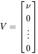
V
=
[
ν
0
⋮
0
]
{\displaystyle V={\begin{bmatrix}\nu \\0\\\vdots \\0\end{bmatrix}}}
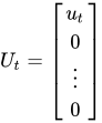
U
t
=
[
u
t
0
⋮
0
]
{\displaystyle U_{t}={\begin{bmatrix}u_{t}\\0\\\vdots \\0\end{bmatrix}}}
where
y
t
{\displaystyle y_{t}}
ν
{\displaystyle \nu }
u
{\displaystyle u}
k
{\displaystyle k}
A
{\displaystyle A}
k
p
{\displaystyle kp}
k
p
{\displaystyle kp}
Y
{\displaystyle Y}
V
{\displaystyle V}
U
{\displaystyle U}
k
p
{\displaystyle kp}
The mean squared error of the h-step forecast of variable
j
{\displaystyle j}
M
S
E
[
y
j
,
t
(
h
)
]
=
∑
i
=
0
h
−
1
∑
l
=
1
k
(
e
j
′
Θ
i
e
l
)
2
=
(
∑
i
=
0
h
−
1
Θ
i
Θ
i
′
)
j
j
=
(
∑
i
=
0
h
−
1
Φ
i
Σ
u
Φ
i
′
)
j
j
,
{\displaystyle \mathbf {MSE} [y_{j,t}(h)]=\sum _{i=0}^{h-1}\sum _{l=1}^{k}(e_{j}'\Theta _{i}e_{l})^{2}={\bigg (}\sum _{i=0}^{h-1}\Theta _{i}\Theta _{i}'{\bigg )}_{jj}={\bigg (}\sum _{i=0}^{h-1}\Phi _{i}\Sigma _{u}\Phi _{i}'{\bigg )}_{jj},}
and where
e
j
{\displaystyle e_{j}}
th column of
I
k
{\displaystyle I_{k}}
j
j
{\displaystyle jj}
Θ
i
=
Φ
i
P
,
{\displaystyle \Theta _{i}=\Phi _{i}P,}
P
{\displaystyle P}
triangular matrix obtained by a Cholesky decomposition of
Σ
u
{\displaystyle \Sigma _{u}}
Σ
u
=
P
P
′
{\displaystyle \Sigma _{u}=PP'}
Σ
u
{\displaystyle \Sigma _{u}}
covariance matrix of the errors
u
t
{\displaystyle u_{t}}
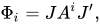
Φ
i
=
J
A
i
J
′
,
{\displaystyle \Phi _{i}=JA^{i}J',}
J
=
[
I
k
0
…
0
]
,
{\displaystyle J={\begin{bmatrix}\mathbf {I} _{k}&0&\dots &0\end{bmatrix}},}
J
{\displaystyle J}
k
{\displaystyle k}
k
p
{\displaystyle kp}
The amount of forecast error variance of variable
j
{\displaystyle j}
l
{\displaystyle l}
ω
j
l
,
h
,
{\displaystyle \omega _{jl,h},}
ω
j
l
,
h
=
∑
i
=
0
h
−
1
(
e
j
′
Θ
i
e
l
)
2
/
M
S
E
[
y
j
,
t
(
h
)
]
.
{\displaystyle \omega _{jl,h}=\sum _{i=0}^{h-1}(e_{j}'\Theta _{i}e_{l})^{2}/MSE[y_{j,t}(h)].}
↑ Lütkepohl, H. (2007) New Introduction to Multiple Time Series Analysis , Springer. p. 63.







![{\displaystyle \mathbf {MSE} [y_{j,t}(h)]=\sum _{i=0}^{h-1}\sum _{l=1}^{k}(e_{j}'\Theta _{i}e_{l})^{2}={\bigg (}\sum _{i=0}^{h-1}\Theta _{i}\Theta _{i}'{\bigg )}_{jj}={\bigg (}\sum _{i=0}^{h-1}\Phi _{i}\Sigma _{u}\Phi _{i}'{\bigg )}_{jj},}](https://wikimedia.org/api/rest_v1/media/math/render/svg/83a54977393cc426642c00435eb061c072deeccb)





![{\displaystyle \omega _{jl,h}=\sum _{i=0}^{h-1}(e_{j}'\Theta _{i}e_{l})^{2}/MSE[y_{j,t}(h)].}](https://wikimedia.org/api/rest_v1/media/math/render/svg/344f3c3885ba18e7782aaaa3068724d6db1143fe)
