Kac's lemma

In ergodic theory, Kac's lemma, demonstrated by mathematician Mark Kac in 1947, is a lemma stating that in a finite measure space the orbit of almost all the points contained in a set $A$ of such space, whose measure is $\mu (A)$, return to $A$ within an average time inversely proportional to $\mu (A)$.

The lemma extends what is stated by Poincaré recurrence theorem, in which it is shown that the points return in $A$ infinite times.

Intuition

In simple terms, it states that for a measure-preserving system, the expected return time to a given subset of the space is inversely proportional to the measure (or size) of that subset. If you have a space with a total measure of 1 (a probability space), and a subset $A$, the average number of steps it takes for points starting in $A$ to return to $A$ for the first time is exactly ${\frac {1}{\mu (A)}}$.

Formal statement

Kac's Lemma—$(X,{\mathcal {B}},\mu ,T)$ be a probability measure-preserving system. This means:

1. $X$ is the state space.
2. $\mu$ is a probability measure on $X$, so $\mu (X)=1$.
3. $T:X\to X$ is a measurable, measure-preserving transformation (i.e., $\mu (T^{-1}(A))=\mu (A)$ for all $A\in {\mathcal {B}}$).
4. The system is assumed to be ergodic (though a version exists for non-ergodic systems, the classic formula holds beautifully for ergodic ones).

Let $A\in {\mathcal {B}}$ be a set with $\mu (A)>0$. For any point $x\in A$, we define the first return time function $\tau _{A}(x)$ as:

$\tau _{A}(x)=\min\{k\geq 1:T^{k}(x)\in A\}$

Then:

$\int _{A}\tau _{A}(x)\,d\mu (x)=1$

We can also look at the conditional expectation (the average return time given that we started in $A$), we divide by $\mu (A)$:

$\mathbb {E} _{A}[\tau _{A}]={\frac {\int _{A}\tau _{A}(x)\,d\mu (x)}{\int _{A}d\mu (x)}}={\frac {1}{\mu (A)}}\int _{A}\tau _{A}(x)\,d\mu (x)$

Or also

$\mathbb {E} _{A}[\tau _{A}]={\frac {1}{\mu (A)}}\int _{A}\tau _{A}(x)\,d\mu (x)\propto {\frac {1}{\mu (A)}}$

Proof

1. Partitioning the Space

Let $E_{k}$ be the set of points in $A$ whose first return to $A$ happens at exactly step $k$:

$E_{k}=\{x\in A:n_{A}(x)=k\}$

By Poincaré Recurrence, almost every point in $A$ returns eventually, so $A=\bigcup _{k=1}^{\infty }E_{k}$ (up to a set of measure zero), and these sets are disjoint. Therefore:

$\int _{A}n_{A}(x)\,d\mu (x)=\sum _{k=1}^{\infty }k\cdot \mu (E_{k})$

2. Shifting the Sets

Now, consider what happens when we apply the transformation $T$. Let's look at the sets $T^{j}(E_{k})$ for $0\leq j<k$.

• $E_{k}$ is in $A$.
• $T(E_{k})$ is outside of $A$ (if $k>1$).
• $T^{2}(E_{k})$ is outside of $A$.
• ...
• $T^{k-1}(E_{k})$ is outside of $A$.
• $T^{k}(E_{k})$ lands back in $A$.

Because $T$ is measure-preserving, shifting these sets doesn't change their measure: $\mu (T^{j}(E_{k}))=\mu (E_{k})$. Furthermore, all the sets in the collection $\{T^{j}(E_{k}):k\geq 1,0\leq j<k\}$ are mutually disjoint almost everywhere, and their union is the entire space $X$ (assuming the system is ergodic, or focusing on the absorbing set generated by $A$).

3. Summing the Total Measure

Since the union of all these disjoint shifted pieces accounts for the entire measure of the accessible space $X$ (and $\mu (X)=1$), we can sum their measures:

$\mu (X)=\sum _{k=1}^{\infty }\sum _{j=0}^{k-1}\mu (T^{j}(E_{k}))$

Because $T$ is measure-preserving, $\mu (T^{j}(E_{k}))=\mu (E_{k})$. The inner sum just adds $\mu (E_{k})$ exactly $k$ times:

$1=\sum _{k=1}^{\infty }k\cdot \mu (E_{k})$

Notice that the right side of this equation is exactly our expression for $\int _{A}n_{A}(x)\,d\mu (x)$.

Thus:

$\int _{A}n_{A}(x)\,d\mu (x)=1$

Dividing both sides by $\mu (A)$ yields the expected return time: ${\frac {1}{\mu (A)}}$. $\blacksquare$

Kakutani-Rokhlin Skyscraper

Instead of focusing purely on the geometric/heuristic "shifting of sets" (as in the classic proof), the Rubinstein-Salzedo approach leverages the transfer operator (or pull-back under $T$) and indicator functions to keep strict track of the arithmetic of the returns.

Proof

Let $(X,{\mathcal {B}},\mu ,T)$ be a probability measure-preserving system, and let $A\in {\mathcal {B}}$ be a set with $\mu (A)>0$. We assume $T$ is ergodic to simplify the domain of return (so the return time $n_{A}(x)$ is finite almost everywhere).

We define the first return time function as before:

$n_{A}(x)=\min\{k\geq 1:T^{k}(x)\in A\}$

1. The Partitioning of the Space

We partition the entire space $X$ into sets based on their relation to $A$ and their future trajectories.

For $i\geq 1$, let $A_{i}$ be the set of points in $A$ whose first return to $A$ occurs at exactly step $i$:

$A_{i}=\{x\in A:n_{A}(x)=i\}$

Since almost every point in $A$ eventually returns, $A=\bigcup _{i=1}^{\infty }A_{i}$ (up to a measure-zero set), and these sets are pairwise disjoint.

Next, we define the "delay" sets $B_{i,j}$ for $i\geq 1$ and $0\leq j<i$. These represent the points in the system that started in $A_{i}$ and have been iterated $j$ times:

$B_{i,j}=T^{j}(A_{i})$

Since $T$ is measure-preserving, we immediately have:

$\mu (B_{i,j})=\mu (A_{i})\quad {\text{for all }}0\leq j<i$

2. Disjointness and Covering of $X$

The core algebraic step is showing that the collection of all these sets:

${\mathcal {P}}=\{B_{i,j}:i\geq 1,0\leq j<i\}$

forms a partition of the entire space $X$ (up to a set of measure zero).

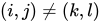
• Disjointness: Suppose $B_{i,j}\cap B_{k,l}\neq \emptyset$ for $(i,j)\neq (k,l)$. This would imply that a point in $A_{i}$ and a point in $A_{k}$ land on the same spot after $j$ and $l$ steps respectively. By tracking this backward to $A$, it would violate the definition of first return times being uniquely $i$ and $k$. Thus, they are pairwise disjoint.
• Covering $X$: By ergodicity, every point in $X$ eventually visits $A$. If a point $y\in X$ takes $m$ steps to hit $A$ for the first time, then $y$ must trace back to some unique start in some $A_{i}$. Hence, $\bigcup _{i=1}^{\infty }\bigcup _{j=0}^{i-1}B_{i,j}=X$ (almost everywhere).

3. Summing the Measures

Since these sets partition $X$, the sum of their measures must equal the total measure of $X$, which is $1$:

$\mu (X)=\sum _{i=1}^{\infty }\sum _{j=0}^{i-1}\mu (B_{i,j})=1$

Substitute $\mu (B_{i,j})=\mu (A_{i})$ into the equation:

$\sum _{i=1}^{\infty }\sum _{j=0}^{i-1}\mu (A_{i})=1$

Because the inner sum does not depend on $j$, we are simply adding $\mu (A_{i})$ exactly $i$ times:

$\sum _{i=1}^{\infty }i\cdot \mu (A_{i})=1$

By definition of the expectation of $n_{A}(x)$ over the set $A$:

$\int _{A}n_{A}(x)\,d\mu =\sum _{i=1}^{\infty }i\cdot \mu (A_{i})=1$

This completes the proof. Dividing by $\mu (A)$ yields the expected return time of ${\frac {1}{\mu (A)}}$. $\blacksquare$

Comparison: Rubinstein-Salzedo vs. The Classic Proof

While both proofs arrive at the same sum, they approach the bookkeeping of the partition from slightly different angles.

Feature	The Classic Proof	Rubinstein-Salzedo Proof
Primary Tool	Pre-images / Pull-backs ($T^{-j}$) Uses inverse maps to pull sets backward.	Forward images ($T^{j}$) Uses forward maps to push sets forward.
Set Definitions	Uses $E_{k}\subseteq A$ and shifts them backward: $T^{-j}(E_{k})$.	Uses $A_{i}\subseteq A$ and pushes them forward: $B_{i,j}=T^{j}(A_{i})$.
Handling of Injectivity	Easier. Pre-images ($T^{-1}$) are automatically well-behaved and preserve disjointness without requiring $T$ to be invertible.	Requires careful handling of the forward map $T^{j}$ (which might not be injective unless $T$ is an invertible/invertible-equivalent system).
Style of Rigor	More standard in classic measure-theory texts (e.g., Walters, Petersen).	Highly algebraic; structured around explicit index-partitioning ($i,j$).

The Rubinstein-Salzedo proof makes the "disjoint skyscraper" structure of the space highly visible. By defining the explicit double-indexed sets $B_{i,j}$, it creates a physical mental model known as a Kakutani-Rokhlin Skyscraper.

In this Skyscraper:

• The set $A$ is the "floor" of the building.
• partition the base by the return time: $A_{k}=\{x\in A:n_{A}(x)=k\}$
• Each $A_{i}$ is a tower base.
• The sets $B_{i,j}=T^{j}(A_{i})$ are the individual floors stacked above $A_{i}$.
• Applying $T$ simply moves you up one floor in the building, until you hit the top floor $B_{i,i-1}$ and get mapped back down to the ground floor $A$.
• tower k is given by $A_{k}\cup T(A_{k})\cup \cdots T^{(k-1)}(A_{k})$ and the measure is given by $\sum _{i=0}^{k-1}\mu (T^{i}(A_{k}))=k\mu (A_{k})$
• each floor of each tower is disjoint $T^{j}(A_{k})\cap T^{m}(A_{k})=\emptyset$ and same is true across towers $T^{i}(A_{m})\cap T^{j}(A_{k})=\emptyset$

This structural visualization makes this approach highly favored for advanced ergodic topics (like holding-time transformations and suspension flows).

Second version

Let $(M,{\mathcal {B}},\mu )$ be a finite measure space. Let $f:M\to M$ be a measurable transformation preserving $\mu$. Let $E\in {\mathcal {B}}$ be any measurable set with positive measure.

Define the first-return time function $\rho _{E}:E\to \mathbb {Z} ^{+}\cup \{\infty \}$ by

$\rho _{E}(x)=\min\{n\geq 1:f^{n}(x)\in E\}$

if this set is nonempty, and otherwise, let it be $\rho _{E}(x)=\infty$ if no iterate of $x$ is in $E$. (Note that by the Poincaré recurrence theorem, the set on the right side is nonempty for almost every point.)

Then one version of Kac's lemma states that $\rho _{E}$ is integrable (i.e. $\rho _{E}\in {\mathcal {L}}^{1}(\mu |_{E})$), with

$\int _{E}\rho _{E}{\text{ d}}\mu =\mu (M)-\mu (E_{0}^{*}).$

This version is provable using elementary measure theory and real analysis. If the system $(f,\mu )$ is in fact ergodic, then the set $E_{0}^{*}$ has zero measure, so, dividing both sides by $\mu (E)$, we indeed get that (almost everywhere in $E$) the mean return time is equal to the measure of the whole space divided by the measure of the set $E$, which is the statement of the lemma.

Application

In physics, a dynamical system evolving in time may be described in a phase space, that is by the evolution in time of some variables. If this variables are bounded, that is having a minimum and a maximum, for a theorem due to Liouville, a measure can be defined in the space, having a measure space where the lemma applies. As a consequence, given a configuration of the system (a point in the phase space) the average return period close to this configuration (in the neighbourhood of the point) is inversely proportional to the considered size of volume surrounding the configuration.

Normalizing the measure space to 1, it becomes a probability space and the measure $P(A)$ of its set $A$ represents the probability of finding the system in the states represented by the points of that set. In this case the lemma implies that the smaller is the probability to be in a certain state (or close to it), the longer is the time of return near that state.

In formulas, if $A$ is the region close to the starting point and $T_{R}$ is the return period, its average value is:

$\langle T_{R}\rangle =\tau /P(A)$

Where $\tau$ is a characteristic time of the system in question.

Note that since the volume of $A$, therefore $P(A)$, depends exponentially on the $n$ variables in the system ($A=\epsilon ^{n}$, with $\epsilon$ infinitesimal side, therefore less than 1, of the volume in $n$ dimensions), $P(A)$ decreases very rapidly as the variables of the system increase and consequently the return period increases exponentially.

In practice, as the variables needed to describe the system increase, the return period increases rapidly.

Further reading

• Kac, Mark (1947). "On the notion of recurrence in discrete stochastic processes" (PDF). Bulletin of the American Mathematical Society. 53 (10): 1002–1010. doi:10.1090/S0002-9904-1947-08927-8.
• Walkden, Charles. "MAGIC: 10 lectures course on ergodic theory – Lecture 5".
• Petersen, Karl E. (1983). Ergodic Theory. Cambridge: Cambridge University Press. p. 46. ISBN 0521236320.
• Hochman, Michael (2013-01-27). "Notes on ergodic theory" (PDF).

Standard Graduate Textbooks

• Petersen, K. (1989). Ergodic Theory. Cambridge University Press.
• Walters, P. (1982). An Introduction to Ergodic Theory. Springer Graduate Texts in Mathematics.
• Einsiedler, M., & Ward, T. (2011). Ergodic Theory: with a view towards Number Theory. Springer Science & Business Media.

Secondary & Survey References

• Krengel, U. (1985). Ergodic Theorems. De Gruyter.
• Shields, P. C. (1996). The Ergodic Theory of Discrete Sample Paths. American Mathematical Society.