Böhm tree

In the study of denotational semantics of the lambda calculus, Böhm trees, Lévy-Longo trees, and Berarducci trees are (potentially infinite) tree-like mathematical objects that capture the "meaning" of a term up to some set of "meaningless" terms.

Motivation

A simple way to read the meaning of a computation is to consider it as a mechanical procedure consisting of a finite number of steps that, when completed, yields a result. In particular, considering the lambda calculus as a rewriting system, each beta reduction step is a rewrite step, and once there are no further beta reductions the term is in normal form. We could thus, naively following Church's suggestion, say the meaning of a term is its normal form, and that terms without a normal form are meaningless. For example, the meanings of $\mathbf {I} =\lambda x.x$ and $\mathbf {II}$ are both $\mathbf {I}$. This works for any strongly normalizing subset of the lambda calculus, such as a typed lambda calculus.

This naive assignment of meaning is however inadequate for the full lambda calculus. The term $\mathbf {\Omega } =(\lambda x.xx)(\lambda x.xx)$ does not have a normal form, and similarly the term $\mathbf {X} =\lambda x.x\mathbf {\Omega }$ does not have a normal form. But the application $\mathbf {\Omega } (\mathbf {KI} )$, where $\mathbf {K}$ denotes the standard lambda term $\lambda x.\lambda y.x$, reduces only to itself, whereas the application $\mathbf {X} (\mathbf {KI} )$ reduces with normal order reduction to $\mathbf {I}$, hence has a meaning. We thus see that not all non-normalizing terms are equivalent. We would like to say that $\mathbf {\Omega }$ is less meaningful than $\mathbf {X}$ because applying $\mathbf {X}$ to a term can produce a result but applying $\mathbf {\Omega }$ cannot.

Böhm trees may also be applied in the context of the infinitary lambda calculus, which includes infinitely large terms. In this context, the term $\mathbf {NN}$, where $\mathbf {N} =\lambda x.\mathbf {I} (xx)$, reduces to both to $\mathbf {I} (\mathbf {I} (\dots ))$ and $\mathbf {\Omega }$, hence there are also issues with confluence of normalization.

Sets of meaningless terms

The general construction is parameterized by a set $U$ of meaningless terms, which is required to satisfy the following axioms:

• Root-activeness: Every root-active term is in $U$. A term $M$ is root-active if for all $M{\stackrel {*}{\to }}N$ there exists a redex $(\lambda x.P)Q$ such that $N{\stackrel {*}{\to }}(\lambda x.P)Q$.
• Closure under β-reduction: For all $M\in U$, if $M{\stackrel {*}{\to }}N$ then $N\in U$.
• Closure under substitution: For all $M\in U$ and substitutions $\sigma$, $M\sigma \in U$.
• Overlap: For all $\lambda x.M\in U$, $(\lambda x.M)N\in U$ .
• Indiscernibility: For all $M,N$, if $N$ can be obtained from $M$ by replacing a set of pairwise disjoint subterms in $U$ with other terms of $U$, then $M\in U$ if and only if $N\in U$.
• Closure under β-expansion. For all $N\in U$, if $M{\stackrel {*}{\to }}N$, then $M\in U$. Some definitions leave this out, but it is useful.

There are infinitely many sets of meaningless terms, but the ones most common in the literature are:

• The set of terms without head normal form
• The set of terms without weak head normal form
• The set of root-active terms, i.e. the terms without top normal form or root normal form. Since root-activeness is assumed, this is the smallest set of meaningless terms.

Note that $\mathbf {\Omega }$ is root-active and therefore $\mathbf {\Omega } \in U$ for every set of meaningless terms $U$.

λ⊥-terms

The set of λ-terms with ⊥ (abbreviated λ⊥-terms) is defined coinductively by the grammar $M=\bot \mid x\mid (\lambda x.M)\mid (MM)$. This corresponds to the standard infinitary lambda calculus plus terms containing $\bot$. Beta-reduction on this set is defined in the standard way. Given a set of meaningless terms $U$, we also define a reduction to bottom: if $M[\bot \mapsto \mathbf {\Omega } ]\in U$ and $M\neq \bot$, then $M\to \bot$. The λ⊥-terms are then considered as a rewriting system with these two rules; thanks to the definition of meaningless terms this rewriting system is confluent and normalizing.

The Böhm-like "tree" for a term may then be obtained as the normal form of the term in this system, possibly in an infinitary "in the limit" sense if the term expands infinitely.

Böhm trees

The Böhm trees are obtained by considering the λ⊥-terms where the set of meaningless terms consists of those without head normal form. More explicitly, the Böhm tree BT(M) of a lambda term M can be computed as follows:

1. BT(M) is $\bot$, if M has no head normal form
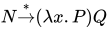
2. $\mathrm {BT} (M)=\lambda x_{1}.\lambda x_{2}.\ldots \lambda x_{n}.y\mathrm {BT} (M_{1})\ldots \mathrm {BT} (M_{m})$, if $M$ reduces in a finite number of steps to the head normal form $\lambda x_{1}.\lambda x_{2}.\ldots \lambda x_{n}.yM_{1}\ldots M_{m}$

For example, $\mathrm {BT} (\mathbf {\Omega } )=\bot$, $\mathrm {BT} (\mathbf {I} )=\mathbf {I}$ and $\mathrm {BT} (\lambda x.x\mathbf {\Omega } )=\lambda x.x\bot$.

Determining whether a term has a head normal form is an undecidable problem. Barendregt introduced a notion of an "effective" Böhm tree that is computable, with the only difference being that terms with no head normal form are not marked with $\bot$.

Note that computing the Böhm tree is similar to finding a normal form for M. If M has a normal form, the Böhm tree is finite and has a simple correspondence to the normal form. If M does not have a normal form, normalization may "grow" some subtrees infinitely, or it may get "stuck in a loop" attempting to produce a result for part of the tree, which produce infinitary trees and meaningless terms respectively. Since the Böhm tree may be infinite the procedure should be understood as being applied co-recursively or as taking the limit of an infinite series of approximations.

Lévy-Longo trees

The Lévy-Longo trees are obtained by considering the λ⊥-terms where the set of meaningless terms consists of those without weak head normal form. More explicitly, the Lévy-Longo tree LLT(M) of a lambda term M can be computed as follows:

1. LLT(M) is $\bot$, if M has no weak head normal form.
2. If $M$ reduces to the weak head normal form $yM_{1}\ldots M_{m}$, then $\mathrm {LLT} (M)=y\mathrm {LLT} (M_{1})\ldots \mathrm {LLT} (M_{m})$.
3. If $M$ reduces to the weak head normal form $\lambda x.N$, then $\mathrm {LLT} (M)=\lambda x.\mathrm {LLT} (N)$/

Berarducci trees

The Berarducci trees are obtained by considering the λ⊥-terms where the set of meaningless terms consists of the root-active terms. More explicitly, the Berarducci tree BerT(M) of a lambda term M can be computed as follows:

1. BerT(M) is $\bot$, if M is root-active.
2. If $M$ reduces to a term $\lambda x.N$, then $\mathrm {BerT} (M)=\lambda x.\mathrm {BerT} (N)$.
3. If $M$ reduces to a term $NP$ where $N$ does not reduce to any abstraction $\lambda x.Q$, then $\mathrm {BerT} (M)=\mathrm {BerT} (N)\mathrm {BerT} (P)$.

References

• Huet, Gérard; Laulhère, H. (1997). "Finite-state Transducers as Regular Böhm Trees" (PDF). In Abadi, M.; Ito, T. (eds.). Theoretical Aspects of Computer Software. LNCS. Vol. 1281. Springer. pp. 604–610. CiteSeerX 10.1.1.110.7910. doi:10.1007/BFb0014570. ISBN 978-3-540-69530-1.
• Gérard Huet (1998). "Regular Böhm Trees" (PDF). Math. Struct. In Comp. Science. 8 (6): 671–680. CiteSeerX 10.1.1.123.475. doi:10.1017/S0960129598002643. S2CID 15752309.
• Ong, C.-H. Luke (31 May 1988). The Lazy Lambda Calculus: An Investigation into the Foundations of Functional Programming (PDF) (PhD). University of London. OCLC 31204528. Retrieved 23 September 2022.
• Sangiorgi, Davide; Walker, David (16 October 2003). The Pi-Calculus: A Theory of Mobile Processes. Cambridge University Press. ISBN 978-0-521-54327-9.
• Barendregt, Henk P. (1977). "The Type Free Lambda Calculus". Handbook of Mathematical Logic. Studies in Logic and the Foundations of Mathematics. Vol. 90. pp. 1091–1132. doi:10.1016/S0049-237X(08)71129-7. hdl:2066/17225. ISBN 9780444863881. S2CID 25828519.
• Severi, Paula; de Vries, Fer-Jan (2011). "Decomposing the Lattice of Meaningless Sets in the Infinitary Lambda Calculus" (PDF). Logic, Language, Information and Computation. Lecture Notes in Computer Science. Vol. 6642. pp. 210–227. doi:10.1007/978-3-642-20920-8_22. ISBN 978-3-642-20919-2. Retrieved 23 September 2022.

References

[edit]- ↑ Levy, Jean-Jacques (1975). "An algebraic interpretation of the λβK-calculus and a labelled λ-calculus". λ-Calculus and Computer Science Theory. Lecture Notes in Computer Science. Vol. 37. pp. 147–165. doi:10.1007/BFb0029523. ISBN 3-540-07416-3.
- ↑ Longo, Giuseppe (August 1983). "Set-theoretical models of λ-calculus: theories, expansions, isomorphisms". Annals of Pure and Applied Logic. 24 (2): 153–188. doi:10.1016/0168-0072(83)90030-1.
- ↑ Berarducci, Alessandro (1996). "Infinite λ-calculus and non-sensible models" (PDF). Logic and algebra. New York: Marcel Dekker. pp. 339–377. ISBN 0824796063. Retrieved 23 September 2007.
- ↑ Church, Alonzo (1941). The calculi of lambda-conversion. Princeton University Press. p. 15. ISBN 0691083940.
{{cite book}}: ISBN / Date incompatibility (help) - ↑ Severi & de Vries 2011, p. 1.
- ↑ Kennaway, Richard; van Oostrom, Vincent; de Vries, Fer-Jan (1996). "Meaningless terms in rewriting". Algebraic and Logic Programming. Lecture Notes in Computer Science. Vol. 1139. pp. 254–268. CiteSeerX 10.1.1.37.3616. doi:10.1007/3-540-61735-3_17. ISBN 978-3-540-61735-8.
- 1 2 Severi & de Vries 2011, p. 5.
- ↑ Severi & de Vries 2011, pp. 4–5.
- ↑ Severi & de Vries 2011, p. 2.
- 1 2 3 Severi & de Vries 2011, p. 6.
- ↑ Barendregt, Henk P. (2012). The Lambda Calculus : Its Syntax and Semantics. London: College Publications. pp. 219–221. ISBN 9781848900660.