// Workers AI · dad joke modeWhy was residual sum of squares sad? It had squared issues.

Not to be confused with the sum of squares due to regression (SSR).

In statistics, the residual sum of squares (RSS), also known as the sum of squared residuals (SSR) or the sum of squared estimate of errors (SSE), is the sum of the squares of residuals (deviations predicted from actual empirical values of data). It is a measure of the discrepancy between the data and an estimation model, such as a linear regression. A small RSS indicates a tight fit of the model to the data. It is used as an optimality criterion in parameter selection and model selection.

In general, total sum of squares = explained sum of squares + residual sum of squares. For a proof of this in the multivariate ordinary least squares (OLS) case, see partitioning in the general OLS model.

One explanatory variable

In a model with a single explanatory variable, RSS is given by:

$$\operatorname {RSS} =\sum _{i=1}^{n}\left(y_{i}-f(x_{i})\right)^{2}$$

where y_i is the i^th value of the variable to be predicted, x_i is the i^th value of the explanatory variable, and $f(x_{i})$ is the predicted value of y_i (also termed ${\hat {y_{i}}}$). In a standard linear simple regression model, $y_{i}=\alpha +\beta x_{i}+\varepsilon _{i}\,$, where $\alpha$ and $\beta$ are coefficients, y and x are the regressand and the regressor, respectively, and ε is the error term. The sum of squares of residuals is the sum of squares of ${\widehat {\varepsilon \,}}_{i}$; that is

$$\operatorname {RSS} =\sum _{i=1}^{n}\left({\widehat {\varepsilon }}_{i}\right)^{2}=\sum _{i=1}^{n}\left(y_{i}-({\widehat {\alpha \,}}+{\widehat {\beta }}\,x_{i})\right)^{2}$$

where ${\widehat {\alpha \,}}$ is the estimated value of the constant term $\alpha$ and ${\widehat {\beta \,}}$ is the estimated value of the slope coefficient $\beta$.

Matrix expression for the OLS residual sum of squares

The general regression model with n observations and k explanators, the first of which is a constant unit vector whose coefficient is the regression intercept, is

$$y=X\beta +e$$

where y is an n × 1 vector of dependent variable observations, each column of the n × k matrix X is a vector of observations on one of the k explanators, $\beta$ is a k × 1 vector of true coefficients, and e is an n× 1 vector of the true underlying errors. The ordinary least squares estimator for $\beta$ is

$${\begin{aligned}&X{\hat {\beta }}=y\\[1ex]\iff &X^{\operatorname {T} }X{\hat {\beta }}=X^{\operatorname {T} }y\\[1ex]\iff &{\hat {\beta }}=\left(X^{\operatorname {T} }X\right)^{-1}X^{\operatorname {T} }y.\end{aligned}}$$

The residual vector ${\hat {e}}=y-X{\hat {\beta }}=y-X(X^{\operatorname {T} }X)^{-1}X^{\operatorname {T} }y$; so the residual sum of squares is:

$$\operatorname {RSS} ={\hat {e}}^{\operatorname {T} }{\hat {e}}=\left\|{\hat {e}}\right\|^{2},$$

(equivalent to the square of the norm of residuals). In full:

$${\begin{aligned}\operatorname {RSS} &=y^{\operatorname {T} }y-y^{\operatorname {T} }X\left(X^{\operatorname {T} }X\right)^{-1}X^{\operatorname {T} }y\\[1ex]&=y^{\operatorname {T} }\left[I-X\left(X^{\operatorname {T} }X\right)^{-1}X^{\operatorname {T} }\right]y\\[1ex]&=y^{\operatorname {T} }\left[I-H\right]y,\end{aligned}}$$

where H is the hat matrix, or the projection matrix in linear regression.

Relation with Pearson's product-moment correlation

The least-squares regression line is given by

$$y=ax+b,$$

where $b={\bar {y}}-a{\bar {x}}$ and $a={\frac {S_{xy}}{S_{xx}}}$, where $S_{xy}=\sum _{i=1}^{n}({\bar {x}}-x_{i})({\bar {y}}-y_{i})$ and $S_{xx}=\sum _{i=1}^{n}({\bar {x}}-x_{i})^{2}.$

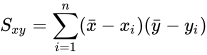
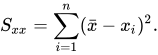
Therefore,

$${\begin{aligned}\operatorname {RSS} &=\sum _{i=1}^{n}\left(y_{i}-f(x_{i})\right)^{2}=\sum _{i=1}^{n}\left(y_{i}-(ax_{i}+b)\right)^{2}\\[1ex]&=\sum _{i=1}^{n}\left(y_{i}-ax_{i}-{\bar {y}}+a{\bar {x}}\right)^{2}=\sum _{i=1}^{n}\left[a\left({\bar {x}}-x_{i}\right)-\left({\bar {y}}-y_{i}\right)\right]^{2}\\[1ex]&=a^{2}S_{xx}-2aS_{xy}+S_{yy}=S_{yy}-aS_{xy}\\[1ex]&=S_{yy}\left(1-{\frac {S_{xy}^{2}}{S_{xx}S_{yy}}}\right)\end{aligned}}$$

where $S_{yy}=\sum _{i=1}^{n}({\bar {y}}-y_{i})^{2}.$

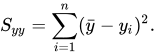
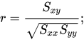
The Pearson product-moment correlation is given by $r={\frac {S_{xy}}{\sqrt {S_{xx}S_{yy}}}};$ therefore, $\operatorname {RSS} =S_{yy}(1-r^{2}).$

See also

• Akaike information criterion § Comparison with least squares
• Chi-squared distribution § Applications
• Degrees of freedom (statistics) § Sum of squares and degrees of freedom
• Errors and residuals in statistics
• Lack-of-fit sum of squares
• Mean squared error
• Reduced chi-squared statistic, RSS per degree of freedom
• Squared deviations
• Sum of squares (statistics)

References

• Draper, N.R.; Smith, H. (1998). Applied Regression Analysis (3rd ed.). John Wiley. ISBN 0-471-17082-8.

References

[edit]- ↑ Archdeacon, Thomas J. (1994). Correlation and regression analysis : a historian's guide. University of Wisconsin Press. pp. 161–162. ISBN 0-299-13650-7. OCLC 27266095.