Multilayer perceptron

In deep learning, a multilayer perceptron (MLP) is a kind of modern feedforward neural network consisting of fully connected neurons with nonlinear activation functions, organized in layers, notable for being able to distinguish data that is not linearly separable.

Modern neural networks are trained using backpropagation and are colloquially referred to as "vanilla" networks. MLPs grew out of an effort to improve on single-layer perceptrons, which could only be applied to linearly separable data. A perceptron traditionally used a Heaviside step function as its nonlinear activation function. However, the backpropagation algorithm requires that modern MLPs use continuous activation functions such as sigmoid or ReLU.

Multilayer perceptrons form the basis of deep learning, and are applicable across a vast set of diverse domains.

Terminology

The name "multilayer perceptron" is a misnomer, as the network relies on neurons with continuous nonlinear activation functions (such as sigmoid, tanh, or rectified linear unit (ReLU)) rather than the Heaviside step function used in the original perceptron. Nevertheless, the name persists to describe feedforward neural networks with at least one hidden layer of fully connected neurons.

In deep learning terminology, MLPs are frequently referred to as deep feedforward networks, feedforward neural networks (FNNs), or simply dense networks. They are also colloquially called "vanilla" neural networks to distinguish them from more specialized architectures. The term "fully connected" distinguishes this architecture, where every neuron in one layer connects to every neuron in the next, from architectures with sparse connectivity such as convolutional neural networks. While the general term "neural network" encompasses all varied architectures (including recurrent and convolutional types), "MLP" specifically denotes the class of feedforward networks with dense connections and no cycles.

Timeline

• In 1943, Warren McCulloch and Walter Pitts proposed the binary artificial neuron as a logical model of biological neural networks.
• In 1958, Frank Rosenblatt proposed the multilayered perceptron model, consisting of an input layer, a hidden layer with randomized weights that did not learn, and an output layer with learnable connections.
• In 1962, Rosenblatt published many variants and experiments on perceptrons in his book Principles of Neurodynamics, including up to 2 trainable layers by "back-propagating errors". However, it was not the backpropagation algorithm, and he did not have a general method for training multiple layers.

• In 1965, Alexey Grigorevich Ivakhnenko and Valentin Lapa published Group Method of Data Handling. It was one of the first deep learning methods, used to train an eight-layer neural net in 1971.

• In 1967, Shun'ichi Amari reported the first multilayered neural network trained by stochastic gradient descent, was able to classify non-linearily separable pattern classes. Amari's student Saito conducted the computer experiments, using a five-layered feedforward network with two learning layers.

• Backpropagation was independently developed multiple times in early 1970s. The earliest published instance was Seppo Linnainmaa's master thesis (1970). Paul Werbos developed it independently in 1971, but had difficulty publishing it until 1982.

• In 1986, David E. Rumelhart et al. popularized backpropagation.

• In 2003, interest in backpropagation networks returned due to the successes of deep learning being applied to language modelling by Yoshua Bengio with co-authors.

• In 2021, a very simple NN architecture combining two deep MLPs with skip connections and layer normalizations was designed and called MLP-Mixer; its realizations featuring 19 to 431 millions of parameters were shown to be comparable to vision transformers of similar size on ImageNet and similar image classification tasks.

Architecture

A multilayer perceptron with full connectivity: every neuron in one layer connects to every neuron in the next layer. This dense architecture allows MLPs to learn arbitrary nonlinear mappings but creates quadratically scaling parameter counts.

A multilayer perceptron is a feedforward neural network, meaning information flows in one direction from input to output with no cycles or loops. Unlike recurrent neural networks, which maintain internal state through feedback connections, or convolutional neural networks, which use sparse local connectivity, MLPs are characterized by full connectivity: every neuron in one layer connects to every neuron in the next layer. This architecture is also called a fully connected network or dense network.

Artificial neuron

Main article: Artificial neuron

Structure of an artificial neuron showing inputs, weights, summation, and activation function.

Each artificial neuron in an MLP receives multiple inputs, processes them through a weighted sum, and applies a nonlinear activation function to produce an output. The neuron model consists of three main parts:

1. Input connections: Each input $x_{i}$ is associated with a synaptic weight $w_{i}$ that represents the strength of that connection. These weights are the learnable parameters of the network.
2. Linear combiner: The neuron computes a weighted sum of its inputs, typically including a bias term $b$:

   $u=\sum _{i=1}^{n}w_{i}x_{i}+b=\mathbf {w} ^{\mathsf {T}}\mathbf {x} +b$

3. Activation function: The weighted sum is passed through a nonlinear function $g(u)$ to produce the neuron's output:

   $y=g(u)=g\left(\sum _{i=1}^{n}w_{i}x_{i}+b\right)$

The bias term can be viewed as an adjustable threshold for neuron activation.

Layer structure

Main article: Layer (deep learning)

The MLP consists of three or more layers: an input layer, one or more hidden layers, and an output layer. The input layer receives the initial data signal (such as pixels of an image or features of a dataset) and passes it to the first hidden layer. It does not perform any computation.

The hidden layers are the computational core of the MLP. Each hidden layer consists of neurons that receive weighted inputs from the previous layer, apply a nonlinear activation function, and pass the result to the next layer. These layers are called "hidden" because their values are not directly observed in the training data, unlike inputs or outputs. Deep networks (those with many hidden layers) can learn hierarchical representations of data: lower layers detect simple features while higher layers represent more abstract concepts.

The output layer produces the final prediction. Its structure depends on the specific task:

• For regression (predicting a continuous value), it typically has a single neuron with a linear activation function.
• For binary classification (predicting yes/no), it uses a single neuron with a sigmoid activation.
• For multi-class classification, it usually has one neuron per class (e.g., 10 neurons for digit recognition), often using the softmax activation to produce a probability distribution.

Connectivity patterns

MLPs are defined by their fully connected (dense) topology: each neuron in layer $i$ connects to every neuron in layer $i+1$. This architecture provides maximum representational flexibility, as the network can learn arbitrary input-output mappings. Using matrix notation, the output $\mathbf {h}$ of a layer with input $\mathbf {x}$ is computed as:

$$\mathbf {h} =\sigma (\mathbf {W} \mathbf {x} +\mathbf {b} ),$$

where $\mathbf {W}$ is the weight matrix, $\mathbf {b}$ is the bias vector, and $\sigma$ is the activation function applied element-wise.

The number of parameters in a fully connected layer equals the product of the input and output dimensions, plus the bias terms. A layer connecting $n$ inputs to $m$ outputs contains $n\times m+m$ learnable parameters. This quadratic scaling means MLPs require substantially more parameters than architectures with sparse connectivity, making them less practical for high-dimensional inputs such as images.

Activation functions

Main article: Activation function

Sigmoid: outputs (0,1)

Tanh: outputs (−1,1)

ReLU: max(0,x)

If a multilayer perceptron has a linear activation function in all neurons, that is, a linear function that maps the weighted inputs to the output of each neuron, then linear algebra shows that any number of layers can be reduced to a two-layer input-output model. In MLPs some neurons must use a nonlinear activation function to learn non-trivial relationships. Early nonlinear activation functions were developed to model the firing frequency of biological neurons.

Common activation functions include:

• Sigmoid, $\sigma (x)=1/(1+e^{-x})$: Historically common, it maps inputs to the range $(0,1)$. It is often used in the output layer for binary classification but is less commonly used in hidden layers due to the vanishing gradient problem.

• Hyperbolic Tangent, $\tanh x$: Similar to the sigmoid but maps inputs to $(-1,1)$. Its zero-centered output often leads to faster convergence than the sigmoid during training.

• Rectified linear unit (ReLU), $f(x)=\max(0,x)$: A common choice for hidden layers. Because its gradient is exactly 1 for positive inputs (and 0 otherwise), ReLU avoids the saturation problem and enables training of deeper networks. The related softplus function provides a smooth approximation.

• Softmax: Typically found in the output layer for multi-class classification. It generalizes the logistic function to multiple dimensions, normalizing a vector of real values into a probability distribution where all values sum to 1.

Mathematical foundations

Activation function

If a multilayer perceptron has a linear activation function in all neurons, that is, a linear function that maps the weighted inputs to the output of each neuron, then linear algebra shows that any number of layers can be reduced to a two-layer input-output model. In MLPs some neurons use a nonlinear activation function that was developed to model the frequency of action potentials, or firing, of biological neurons.

The two historically common activation functions are both sigmoids, and are described by

$y(v_{i})=\tanh(v_{i})~~{\textrm {and}}~~y(v_{i})=(1+e^{-v_{i}})^{-1}$.

The first is a hyperbolic tangent that ranges from −1 to 1, while the other is the logistic function, which is similar in shape but ranges from 0 to 1. Here $y_{i}$ is the output of the $i$th node (neuron) and $v_{i}$ is the weighted sum of the input connections. Alternative activation functions have been proposed, including the rectifier and softplus functions. More specialized activation functions include radial basis functions (used in radial basis networks, another class of supervised neural network models).

In recent developments of deep learning the rectified linear unit (ReLU) is more frequently used as one of the possible ways to overcome the numerical problems related to the sigmoids.

Layers

Main article: Layer (deep learning)

The MLP consists of three or more layers (an input and an output layer with one or more hidden layers) of nonlinearly-activating nodes. Since MLPs are fully connected, each node in one layer connects with a certain weight $w_{ij}$ to every node in the following layer.

Learning

Learning occurs in the perceptron by changing connection weights after each piece of data is processed, based on the amount of error in the output compared to the expected result. This is an example of supervised learning, and is carried out through backpropagation, a generalization of the least mean squares algorithm in the linear perceptron.

We can represent the degree of error in an output node $j$ in the $n$th data point (training example) by $e_{j}(n)=d_{j}(n)-y_{j}(n)$, where $d_{j}(n)$ is the desired target value for $n$th data point at node $j$, and $y_{j}(n)$ is the value produced by the perceptron at node $j$ when the $n$th data point is given as an input.

The node weights can then be adjusted based on corrections that minimize the error in the entire output for the $n$th data point, given by

${\mathcal {E}}(n)={\frac {1}{2}}\sum _{{\text{output node }}j}e_{j}^{2}(n)$.

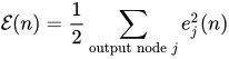
Using gradient descent, the change in each weight $w_{ij}$ is

$\Delta w_{ji}(n)=-\eta {\frac {\partial {\mathcal {E}}(n)}{\partial v_{j}(n)}}y_{i}(n)$

where $y_{i}(n)$ is the output of the previous neuron $i$, and $\eta$ is the learning rate, which is selected to ensure that the weights quickly converge to a response, without oscillations. In the previous expression, ${\frac {\partial {\mathcal {E}}(n)}{\partial v_{j}(n)}}$ denotes the partial derivate of the error ${\mathcal {E}}(n)$ according to the weighted sum $v_{j}(n)$ of the input connections of neuron $i$.

The derivative to be calculated depends on the induced local field $v_{j}$, which itself varies. It is easy to prove that for an output node this derivative can be simplified to

$-{\frac {\partial {\mathcal {E}}(n)}{\partial v_{j}(n)}}=e_{j}(n)\phi ^{\prime }(v_{j}(n))$

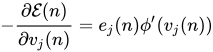
where $\phi ^{\prime }$ is the derivative of the activation function described above, which itself does not vary. The analysis is more difficult for the change in weights to a hidden node, but it can be shown that the relevant derivative is

$-{\frac {\partial {\mathcal {E}}(n)}{\partial v_{j}(n)}}=\phi ^{\prime }(v_{j}(n))\sum _{k}-{\frac {\partial {\mathcal {E}}(n)}{\partial v_{k}(n)}}w_{kj}(n)$.

This depends on the change in weights of the $k$th nodes, which represent the output layer. So to change the hidden layer weights, the output layer weights change according to the derivative of the activation function, and so this algorithm represents a backpropagation of the activation function.

Training

Main articles: Backpropagation and Stochastic gradient descent

The iterative training loop: each step performs forward propagation to compute predictions and loss, backpropagation to compute gradients, and a parameter update. Training continues until convergence criteria are met.

Learning in an MLP occurs by adjusting connections (weights) and biases to minimize a loss function, which measures the discrepancy between predictions and targets. This is typically achieved using backpropagation to compute gradients combined with stochastic gradient descent (SGD) or its variants.

Training proceeds iteratively over minibatches sampled from the training dataset. In each iteration, a minibatch of input-target pairs $(\mathbf {x} ,y)$ is processed through two phases: a forward pass and a backward pass. The forward pass computes predictions ${\hat {y}}$ from the inputs and evaluates the loss function $L({\hat {y}},y)$, which quantifies the error between predictions and targets. The backward pass computes gradients of the loss with respect to all parameters—denoted collectively as $\theta$ (encompassing all weights and biases)—using the chain rule of calculus. These gradients $\nabla _{\theta }L$ indicate the direction to adjust parameters to reduce the loss. Finally, parameters are updated using the rule $\theta \leftarrow \theta -\eta \nabla _{\theta }L$, where $\eta$ is the learning rate controlling the step size.

At a finer level of detail, for a weight connecting neuron $j$ in one layer to neuron $i$ in the next, the gradient is proportional to the error term $\delta _{i}$ (the sensitivity of the loss to neuron $i$'s activation) and the activation $h_{j}$ from the previous layer. Training often utilizes adaptive optimization algorithms like Adam and RMSProp, which modify the basic SGD update rule to adapt the learning rate for each parameter individually, accelerating convergence and improving stability.

Training deep networks presents specific challenges. The vanishing gradient problem, identified by Sepp Hochreiter in 1991 and further analyzed by Bengio et al., occurs when sigmoidal activations saturate. Saturated activations produce near-zero derivatives; these small values multiply across layers, causing error signals to diminish exponentially. ReLU activations address this problem: unlike sigmoidal units, rectified linear units preserve information as it travels through multiple layers. Proper initialization is also critical; techniques like Glorot initialization and He initialization scale initial weights to preserve signal variance.

To prevent overfitting, regularization techniques are standard. Weight decay ($L^{2}$ regularization) adds a penalty for large weights, while dropout randomly disables a fraction of neurons during each training step to enforce robust representations. Early stopping halts training if validation performance degrades. Although the loss landscape is non-convex with multiple local minima, theoretical analysis suggests that in sufficiently large networks, most local minima achieve error rates comparable to global minima.

Applications

Main article: Artificial neural network § Applications

For structured tabular data—the heterogeneous rows and columns typical of financial, medical, and industrial datasets—MLPs remain competitive with specialized methods. A 2021 study found that properly regularized deep MLP architectures can be competitive with gradient-boosted decision trees, which have traditionally dominated this domain. Unlike decision trees, MLPs are differentiable and can be trained end-to-end in multi-modal pipelines that combine tabular features with images or text.

In the physical and atmospheric sciences, MLPs serve as surrogate models that approximate computationally expensive simulations at lower cost. Because MLPs can approximate continuous functions on compact domains (as guaranteed by the universal approximation theorem), they can learn to replicate the input-output behavior of complex physical systems at a fraction of the computational cost. This enables rapid iterative analysis and real-time forecasting in domains such as weather prediction, fluid dynamics, and materials science.

MLPs are also used in large-scale recommender systems to model complex interactions between user history and content features. Beyond these standalone applications, MLPs serve as components within larger architectures, forming the classification heads of convolutional neural networks and the position-wise feed-forward networks within Transformers (see below).

Relationship with other architectures

In deep learning, the MLP functions as a building block within larger architectures. The Transformer architecture, which underlies large language models and foundation models, incorporates MLPs as position-wise feed-forward networks in every encoder and decoder layer. Unlike the attention mechanism, which aggregates information across sequence positions, these feed-forward components operate on each position independently, consisting of two linear transformations with a ReLU activation.

Similarly, convolutional neural networks typically employ fully connected MLP layers as a classification head. After convolutional and pooling layers extract hierarchical spatial features, the resulting feature maps are flattened and passed through one or more dense layers that integrate these features to produce class predictions. While the convolutional layers provide translation invariance and local connectivity, the MLP layers perform the final combinatorial logic required to map features to output categories.

The MLP-Mixer architecture, introduced in 2021, demonstrated that models composed entirely of MLP layers—without convolution or self-attention—can achieve competitive performance on image classification benchmarks when trained on sufficiently large datasets. This work showed that the inductive biases of specialized architectures, while helpful for data efficiency, are not strictly necessary for strong performance when sufficient data is available.

Historically, the relationship between MLPs and other methods was framed more competitively. The MLP overcame the fundamental limitation of single-layer perceptrons, which Minsky and Papert proved incapable of learning non-linearly separable functions such as XOR. In the 1990s, MLPs competed directly with support vector machines, which offered convex optimization guarantees that MLPs lacked; however, MLPs scaled better to large datasets through stochastic gradient descent and could be stacked into deeper architectures.

Limitations

The fully connected structure that gives MLPs their flexibility also introduces inefficiencies for certain data types. Because every neuron connects to every neuron in adjacent layers, the number of parameters scales quadratically with layer dimensions—a layer connecting $n$ inputs to $m$ outputs requires $n\times m$ weights plus bias terms. For high-dimensional inputs such as images, this scaling becomes prohibitively expensive and increases the risk of overfitting, particularly when training data is limited. Architectures like convolutional neural networks address this through weight sharing and local receptive fields, significantly reducing parameter counts for spatially structured data.

MLPs lack the inductive biases that allow specialized architectures to learn efficiently from limited data. They treat input features as independent of one another, ignoring spatial relationships that convolutional neural networks exploit through local connectivity and translation invariance. Similarly, MLPs process fixed-size inputs without internal mechanisms for handling variable-length sequences or temporal dependencies, unlike recurrent neural networks or Transformers. Consequently, MLPs must learn structural regularities entirely from training examples, requiring substantially more data to achieve comparable performance on tasks where such structure exists.

Like other deep neural networks, MLPs function as "black boxes" whose decision-making processes are difficult to interpret. Unlike linear models or decision trees, where the influence of individual input variables is explicit, MLPs distribute learned representations across many nonlinear hidden units. This makes it challenging to understand how specific outputs are derived from inputs, limiting their applicability in domains where interpretability is required.

External links

• Weka: Open source data mining software with multilayer perceptron implementation.
• Neuroph Studio documentation, implements this algorithm and a few others.

References

[edit]- ↑ Cybenko, G. 1989. Approximation by superpositions of a sigmoidal function Mathematics of Control, Signals, and Systems, 2(4), 303–314.
- ↑ Linnainmaa, Seppo (1970). The representation of the cumulative rounding error of an algorithm as a Taylor expansion of the local rounding errors (Masters) (in Finnish). University of Helsinki. pp. 6–7.
- ↑ Kelley, Henry J. (1960). "Gradient theory of optimal flight paths". ARS Journal. 30 (10): 947–954. doi:10.2514/8.5282.
- ↑ Rosenblatt, Frank. x. Principles of Neurodynamics: Perceptrons and the Theory of Brain Mechanisms. Spartan Books, Washington DC, 1961
- ↑ Werbos, Paul (1982). "Applications of advances in nonlinear sensitivity analysis" (PDF). System modeling and optimization. Springer. pp. 762–770. Archived (PDF) from the original on 14 April 2016. Retrieved 2 July 2017.
- ↑ Rumelhart, David E., Geoffrey E. Hinton, and R. J. Williams. "Learning Internal Representations by Error Propagation". David E. Rumelhart, James L. McClelland, and the PDP research group. (editors), Parallel distributed processing: Explorations in the microstructure of cognition, Volume 1: Foundation. MIT Press, 1986.
- ↑ Hastie, Trevor. Tibshirani, Robert. Friedman, Jerome. The Elements of Statistical Learning: Data Mining, Inference, and Prediction. Springer, New York, NY, 2009.
- ↑ "Why is the ReLU function not differentiable at x=0?". 21 November 2024.
- ↑ Almeida, Luis B (2020) [1996]. "Multilayer perceptrons". In Fiesler, Emile; Beale, Russell (eds.). Handbook of Neural Computation. CRC Press. pp. C1-2. doi:10.1201/9780429142772. ISBN 978-0-429-14277-2.
- 1 2 Gardner, Matt W; Dorling, Stephen R (1998). "Artificial neural networks (the multilayer perceptron)—a review of applications in the atmospheric sciences". Atmospheric Environment. 32 (14–15). Elsevier: 2627–2636. Bibcode:1998AtmEn..32.2627G. doi:10.1016/S1352-2310(97)00447-0. Cite error: The named reference "AtmosSciPaper" was defined multiple times with different content (see the help page).
- 1 2 3 4 Bishop, Christopher M. (2006). Pattern Recognition and Machine Learning. Springer. ISBN 978-0-387-31073-2. Retrieved 2026-01-04.
- ↑ Hornik, Kurt (1991). "Approximation capabilities of multilayer feedforward networks". Neural Networks. 4 (2): 251–257. doi:10.1016/0893-6080(91)90009-T.
- 1 2 3 4 5 6 7 8 9 10 11 12 13 14 15 16 17 Goodfellow, Ian; Bengio, Yoshua; Courville, Aaron (2016). "6. Deep Feedforward Networks". Deep Learning. MIT Press. pp. 163–200. ISBN 978-0-262-03561-3. Retrieved 2026-01-04.: 163–168
- ↑ Hastie, Trevor; Tibshirani, Robert; Friedman, Jerome (2009). The Elements of Statistical Learning: Data Mining, Inference, and Prediction (2nd ed.). Springer. ISBN 978-0-387-84857-0. Retrieved 2026-01-04.: 389–416
- ↑ McCulloch, Warren S.; Pitts, Walter (1943-12-01). "A logical calculus of the ideas immanent in nervous activity". The Bulletin of Mathematical Biophysics. 5 (4): 115–133. doi:10.1007/BF02478259. ISSN 1522-9602.
- ↑ Rosenblatt, Frank (1958). "The Perceptron: A Probabilistic Model For Information Storage And Organization in the Brain". Psychological Review. 65 (6): 386–408. doi:10.1037/h0042519. PMID 13602029. S2CID 12781225.
- ↑ Rosenblatt, Frank (1962). Principles of Neurodynamics. Spartan, New York.
- ↑ Ivakhnenko, A. G. (1973). Cybernetic Predicting Devices. CCM Information Corporation.
- ↑ Ivakhnenko, A. G.; Grigorʹevich Lapa, Valentin (1967). Cybernetics and forecasting techniques. American Elsevier Pub. Co.
- 1 2 3 Schmidhuber, Juergen (2022). "Annotated History of Modern AI and Deep Learning". arXiv:2212.11279 [cs.NE].
- ↑ Amari, Shun'ichi (1967). "A theory of adaptive pattern classifier". IEEE Transactions. EC (16): 279-307.
- ↑ Linnainmaa, Seppo (1970). The representation of the cumulative rounding error of an algorithm as a Taylor expansion of the local rounding errors (Masters) (in Finnish). University of Helsinki. p. 6–7.
- ↑ Linnainmaa, Seppo (1976). "Taylor expansion of the accumulated rounding error". BIT Numerical Mathematics. 16 (2): 146–160. doi:10.1007/bf01931367. S2CID 122357351.
- ↑ Anderson, James A.; Rosenfeld, Edward, eds. (2000). Talking Nets: An Oral History of Neural Networks. The MIT Press. doi:10.7551/mitpress/6626.003.0016. ISBN 978-0-262-26715-1.
- ↑ Rumelhart, David E.; Hinton, Geoffrey E.; Williams, Ronald J. (October 1986). "Learning representations by back-propagating errors". Nature. 323 (6088): 533–536. Bibcode:1986Natur.323..533R. doi:10.1038/323533a0. ISSN 1476-4687.
- ↑ Bengio, Yoshua; Ducharme, Réjean; Vincent, Pascal; Janvin, Christian (March 2003). "A neural probabilistic language model". The Journal of Machine Learning Research. 3: 1137–1155.
- ↑ "Papers with Code – MLP-Mixer: An all-MLP Architecture for Vision".
- 1 2 3 Haykin, Simon (1998). Neural Networks: A Comprehensive Foundation (2nd ed.). Prentice Hall. ISBN 0-13-273350-1.
- ↑ Wasserman, Philip D. (1989). Neural Computing: Theory and Practice. New York: Van Nostrand Reinhold. ISBN 0-442-20743-3.
- ↑ Almeida, Luis B. (1996). "Multilayer Perceptrons". In Fiesler, Emile; Beale, Russell (eds.). Handbook of Neural Computation. Oxford University Press. ISBN 978-0750303125.
- ↑ LeCun, Yann; Bottou, Léon; Orr, Genevieve B.; Müller, Klaus-Robert (2012). "Efficient BackProp". Neural Networks: Tricks of the Trade. Springer. pp. 9–48. ISBN 978-3-642-35288-1.
- 1 2 Nair, Vinod; Hinton, Geoffrey E. (2010). Rectified Linear Units Improve Restricted Boltzmann Machines (PDF). Proceedings of the 27th International Conference on Machine Learning. pp. 807–814. Retrieved 2026-01-05.
- ↑ Haykin, Simon (1998). Neural Networks: A Comprehensive Foundation (2 ed.). Prentice Hall. ISBN 0-13-273350-1.
- ↑ Kingma, Diederik P.; Ba, Jimmy (2015). Adam: A Method for Stochastic Optimization. International Conference on Learning Representations. arXiv:1412.6980.
- 1 2 Gorishniy, Yury; Rubachev, Ivan; Khrulkov, Valentin; Babenko, Artem (2021). Revisiting Deep Learning Models for Tabular Data (PDF). Advances in Neural Information Processing Systems. Vol. 34. pp. 18932–18943. Retrieved 2026-01-03.
- ↑ Cite error: The named reference
Schmidhuber2022was invoked but never defined (see the help page). - ↑ Bengio, Yoshua; Simard, Patrice; Frasconi, Paolo (1994). "Learning long-term dependencies with gradient descent is difficult". IEEE Transactions on Neural Networks. 5 (2): 157–166. doi:10.1109/72.279181.
- 1 2 Cite error: The named reference
Glorot2010was invoked but never defined (see the help page). - ↑ Srivastava, Nitish; Hinton, Geoffrey; Krizhevsky, Alex; Sutskever, Ilya; Salakhutdinov, Ruslan (2014). "Dropout: A Simple Way to Prevent Neural Networks from Overfitting". Journal of Machine Learning Research. 15: 1929–1958. Retrieved 2026-01-04.
- ↑ Choromanska, Anna; Henaff, Mikael; Mathieu, Michael; Ayesha, Ben; LeCun, Yann (2015). The Loss Surfaces of Multilayer Networks. International Conference on Artificial Intelligence and Statistics. arXiv:1412.0233.
- ↑ Covington, Paul; Adams, Jay; Sargin, Emre (2016). Deep Neural Networks for YouTube Recommendations. Proceedings of the 10th ACM Conference on Recommender Systems. pp. 191–198. doi:10.1145/2959100.2959190.
Vaswani2017was invoked but never defined (see the help page). - ↑ Cite error: The named reference
Tolstikhin2021was invoked but never defined (see the help page). - ↑ Cite error: The named reference
Minsky1969was invoked but never defined (see the help page).