// Workers AI · dad joke modeWhat did the binomial options pricing model say? "I've got a binary decision to make.

In finance, the binomial options pricing model is a lattice-based numerical method for valuing options. It represents possible prices of the underlying instrument on a discrete-time binomial tree and values the option by backward induction. Because exercise decisions can be evaluated at individual nodes, the method is particularly useful for American and Bermudan options.

William F. Sharpe presented a binomial option-pricing procedure in the 1978 edition of Investments. John Cox, Stephen Ross and Mark Rubinstein published a widely used formulation in 1979, and Richard Rendleman Jr. and Brit Bartter published a separate two-state formulation in the same year.

For binomial trees applied to fixed income and interest rate derivatives, see Lattice model (finance) § Interest rate derivatives.

Use of the model

The Binomial options pricing model approach has been widely used since it is able to handle a variety of conditions for which other models cannot easily be applied. This is largely because the BOPM is based on the description of an underlying instrument over a period of time rather than a single point. As a consequence, it is used to value American options that are exercisable at any time in a given interval as well as Bermudan options that are exercisable at specific instances of time. Being relatively simple, the model is readily implementable in computer software (including a spreadsheet).

Although higher in computational complexity and computationally slower than the Black–Scholes formula, it is more accurate, particularly for longer-dated options on securities with dividend payments. For these reasons, various versions of the binomial model are widely used by practitioners in the options markets.

For options with several sources of uncertainty (e.g., real options) and for options with complicated features (e.g., Asian options), binomial methods could be less practical due to several difficulties, and Monte Carlo option models are commonly used instead. Monte Carlo simulation is also less susceptible to sampling errors, since binomial techniques use discrete time units. This becomes more true the smaller the discrete units become.

In a non-recombinant binomial tree, in which paths moving in opposite directions do not merge, resulting in unique nodes for every sequence of price changes, the worst-case runtime of BOPM would be O(2ⁿ), where n is the number of time steps in the simulation. Monte Carlo simulation generally has a polynomial time complexity, and would be faster for large numbers of simulation steps, while when simulating a small number of time steps, Monte Carlo simulation would be more computationally intensive than BOPM (cf. Monte Carlo methods in finance). However, in a standard recombinant tree, a down move followed by an up move reaches the same node as an up move followed by a down move. An N-step tree therefore has $(N+1)(N+2)/2$ distinct nodes, so straightforward backward induction has quadratic rather than exponential computational complexity.

Method

Binomial Lattice with CRR formulae

Incorrect code, p[i] is overwritten used in calculation p[i-1], introduce another temp vector to save function americanPut(T, S, K, r, sigma, q, n) { ' T... expiration time ' S... stock price ' K... strike price ' r... interest rate ' sigma... volatility of the stock price ' q... dividend yield ' n... height of the binomial tree deltaT := T / n; up := exp(sigma * sqrt(deltaT)); p0 := (up * exp(-q * deltaT) - exp(-r * deltaT)) / (up^2 - 1); p1 := exp(-r * deltaT) - p0; ' initial values at time T for i := 0 to n { p[i] := K - S * up^(2*i - n+1); if p[i] < 0 then p[i] := 0; } ' move to earlier times for j := n-1 down to 0 { for i := 0 to j { ' binomial value p[i] := p0 * p[i+1] + p1 * p[i]; ' exercise value exercise := K - S * up^(2*i - j); if p[i] < exercise then p[i] := exercise; } } return americanPut := p[0]; }

The binomial pricing model traces the evolution of the option's key underlying variables in discrete-time. This is done by means of a binomial lattice (Tree), for a number of time steps between the valuation and expiration dates. Each node in the lattice represents a possible price of the underlying at a given point in time.

Valuation is performed iteratively, starting at each of the final nodes (those that may be reached at the time of expiration), and then working backwards through the tree towards the first node (valuation date). The value computed at each stage is the value of the option at that point in time.

Option valuation using this method is, as described, a three-step process:

1. Price tree generation,
2. Calculation of option value at each final node,
3. Sequential calculation of the option value at each preceding node.

Step 1: Create the binomial price tree

The tree of prices is produced by working forward from valuation date to expiration.

At each step, it is assumed that the underlying instrument will move up or down by a specific factor ($u$ or $d$) per step of the tree (where, by definition, $u\geq 1$ and $0<d\leq 1$). So, if $S$ is the current price, then in the next period the price will either be $S_{up}=S\cdot u$ or $S_{down}=S\cdot d$.

The up and down factors are calculated using the underlying (fixed) volatility, $\sigma$, and the time duration of a step, $t$, measured in years (using the day count convention of the underlying instrument). From the condition that the variance of the log of the price is $\sigma ^{2}t$, we have:

$u=e^{\sigma {\sqrt {\Delta t}}}$

$d=e^{-\sigma {\sqrt {\Delta t}}}={\frac {1}{u}}.$

Above is the original Cox, Ross, & Rubinstein (CRR) method; there are various other techniques for generating the lattice, such as "the equal probabilities" tree.

The CRR method ensures that the tree is recombinant, i.e. if the underlying asset moves up and then down (u,d), the price will be the same as if it had moved down and then up (d,u)—here the two paths merge or recombine. This property reduces the number of tree nodes, and thus accelerates the computation of the option price.

This property also allows the value of the underlying asset at each node to be calculated directly via formula, and does not require that the tree be built first. The node-value will be:

$S_{n}=S_{0}\times u^{N_{u}-N_{d}},$

Where $N_{u}$ is the number of up ticks and $N_{d}$ is the number of down ticks.

Step 2: Find option value at each final node

At each final node of the tree—i.e. at expiration of the option—the option value is simply its intrinsic, or exercise, value:

Max [ (S_n − K), 0 ], for a call option

Max [ (K − S_n), 0 ], for a put option,

Where K is the strike price and $S_{n}$ is the spot price of the underlying asset at the n^th period.

Step 3: Find option value at earlier nodes

Once the above step is complete, the option value is then found for each node, starting at the penultimate time step, and working back to the first node of the tree (the valuation date) where the calculated result is the value of the option.

In overview: the "binomial value" is found at each node, using the risk neutrality assumption; see Risk neutral valuation. If exercise is permitted at the node, then the model takes the greater of binomial and exercise value at the node.

The steps are as follows:

1. Under the risk neutrality assumption, today's fair price of a derivative is equal to the expected value of its future payoff discounted by the risk free rate. Therefore, expected value is calculated using the option values from the later two nodes (Option up and Option down) weighted by their respective (fixed) probabilities—"probability" p of an up move in the underlying, and "probability" (1−p) of a down move. The expected value is then discounted at r, the risk free rate corresponding to the life of the option.

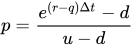
   The following formula to compute the expectation value is applied at each node:

   ${\text{ Binomial Value }}=[p\times {\text{ Option up }}+(1-p)\times {\text{ Option down] }}\times \exp(-r\times \Delta t)$, or

   $C_{t-\Delta t,i}=e^{-r\Delta t}(pC_{t,i}+(1-p)C_{t,i+1})\,$

   where

   $C_{t,i}\,$ is the option's value for the $i^{th}\,$ node at time t,

   $p={\frac {e^{(r-q)\Delta t}-d}{u-d}}$ is chosen such that the related binomial distribution simulates the geometric Brownian motion of the underlying stock with parameters r and σ,

   q is the dividend yield of the underlying corresponding to the life of the option. It follows that in a risk-neutral world futures price should have an expected growth rate of zero and therefore we can consider $q=r$ for futures.

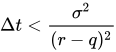
   Note that for p to be in the interval $(0,1)$ the following condition on $\Delta t$ has to be satisfied $\Delta t<{\frac {\sigma ^{2}}{(r-q)^{2}}}$.

   (Note that the alternative valuation approach, arbitrage-free pricing, yields identical results; see “delta-hedging”.)

2. This result is the "Binomial Value". It represents the fair price of the derivative at a particular point in time (i.e. at each node), given the evolution in the price of the underlying to that point. It is the value of the option if it were to be held—as opposed to exercised at that point.
3. Depending on the style of the option, evaluate the possibility of early exercise at each node: if (1) the option can be exercised, and (2) the exercise value exceeds the Binomial Value, then (3) the value at the node is the exercise value.
   • For a European option, there is no option of early exercise, and the binomial value applies at all nodes.
   • For an American option, since the option may either be held or exercised prior to expiry, the value at each node is: Max (Binomial Value, Exercise Value).
   • For a Bermudan option, the value at nodes where early exercise is allowed is: Max (Binomial Value, Exercise Value); at nodes where early exercise is not allowed, only the binomial value applies.

In calculating the value at the next time step calculated—i.e. one step closer to valuation—the model must use the value selected here, for "Option up"/"Option down" as appropriate, in the formula at the node. The aside algorithm demonstrates the approach computing the price of an American put option, although is easily generalized for calls and for European and Bermudan options. For European options in particular, it has been shown that the general binomial-lattice valuation model cannot be represented by a single hypergeometric closed-form expression.

Relationship with Black–Scholes

Similar assumptions underpin both the binomial model and the Black–Scholes-Merton model. Under the Cox–Ross–Rubinstein specification with constant interest rate, dividend yield and volatility, the binomial tree is a discrete time approximation to the geometric Brownian motion used in the Black–Scholes–Merton model. The binomial model assumes that movements in the price follow a binomial distribution; as the number of time steps increases, the distribution of the logarithm of the underlying price approaches a normal distribution and the underlying price approaches a log-normal distribution. Consequently, the value of a European option calculated with the binomial model converges to its Black–Scholes–Merton value.

Convergence need not be monotonic: calculated prices can oscillate as the number of time steps changes, and convergence speed depends on the chosen tree specification and implementation.

When viewed as a numerical procedure, the CRR method can also be interpreted as a special case of the explicit finite difference method for the Black–Scholes partial differential equation; see finite difference methods for option pricing.

See also

• Trinomial tree, a similar model with three possible paths per node.
• Tree (data structure)
• Lattice model (finance), for more general discussion and application to other underlyings
• Black–Scholes: binomial lattices are able to handle a variety of conditions for which Black–Scholes cannot be applied.
• Monte Carlo option model, used in the valuation of options with complicated features that make them difficult to value through other methods.
• Real options analysis, where the BOPM is widely used.
• Quantum finance, quantum binomial pricing model.
• Mathematical finance, which has a list of related articles.
• Employee stock option § Valuation, where the BOPM is widely used.
• Implied binomial tree
• Edgeworth binomial tree

External links

• The Binomial Model for Pricing Options, Prof. Thayer Watkins
• Binomial Option Pricing (PDF), Prof. Robert M. Conroy
• Binomial Option Pricing Model by Fiona Maclachlan, The Wolfram Demonstrations Project
• On the Irrelevance of Expected Stock Returns in the Pricing of Options in the Binomial Model: A Pedagogical Note by Valeri Zakamouline
• A Simple Derivation of Risk-Neutral Probability in the Binomial Option Pricing Model by Greg Orosi

References

[edit]- ↑ Georgiadis, Evangelos (2011). "Binomial options pricing has no closed-form solution". Algorithmic Finance. 1 (1). IOS Press: 11–18. doi:10.3233/AF-2011-003.
- ↑ William F. Sharpe, Biographical, nobelprize.org
- ↑ Cox, J. C.; Ross, S. A.; Rubinstein, M. (1979). "Option pricing: A simplified approach". Journal of Financial Economics. 7 (3): 229. doi:10.1016/0304-405X(79)90015-1.
- ↑ Richard J. Rendleman, Jr. and Brit J. Bartter. 1979. "Two-State Option Pricing". Journal of Finance 24: 1093-1110. doi:10.2307/2327237
- ↑ Gerbessiotis, Alexandros V. (2004). "Architecture independent parallel binomial tree option price valuations". Parallel Computing. 30 (2): 301–316. doi:10.1016/j.parco.2003.09.003.
- 1 2 3 Joshi, Mark S. (2009). "The convergence of binomial trees for pricing the American put". The Journal of Risk. 11 (4): 87–108. doi:10.21314/JOR.2009.197.
- 1 2 Chance, Don M. (2008). "A Synthesis of Binomial Option Pricing Models for Lognormally Distributed Assets". Journal of Applied Finance. 18 (1): 38–56. SSRN 969834.
- ↑ Rubinstein, Mark (2000). "On the Relation Between Binomial and Trinomial Option Pricing Models". The Journal of Derivatives. 8 (2): 47–50. doi:10.3905/jod.2000.319149.